How to correct spelling mistakes while analyzing data?

Grouping in Pivot table is one method of spelling mistakes correction. Here is another option for correcting mistakes using VLOOKUP.

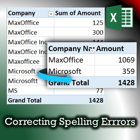
Estimated reading time 10 min

Estimated Time Saving many hours!

Problem: Spelling mistakes or variations

Data will never be perfect. We have to live with it. That does not mean we waste our precious time correcting mistakes. There are faster and smarter ways of handling this problem.

There are two kind of mistakes. Spelling Mistakes and Spelling Variations.

The right spelling is MaxOffice. Mistakes could be MaxxOffice, MaxOfice, MaxOffic

Spelling variations happen because of abbreviations. Maxoffice Ltd, Maxoffice Limited, MaxOffice Inc, MaxOffice Inc. , MaxOffice Incorporated

In either case, it makes analysis difficult because instead of one entry, multiple entries appear in Pivot Table.

There are many ways of handling this situation.

1. Grouping Text in Pivot Tables (Read this article)
2. Vlookup (this article)
3. Master table in Power Pivot (will be covered in a separate article)

Which method to use?

If there are few mistakes, use Grouping in Pivot Tables.

If you expect same or similar data (with similar errors) to be received periodically, then Vlookup or Power Pivot are better options.

If you don’t know / don’t have Power Pivot, use Vlookup option.

Download Sample Files

Unzip the file. There are two files. Base.xlsx and Incremental.xlsx

Look at the raw data in base file. There are only two columns. Company and Amount. Company column has spelling mistakes and spelling variations.

To make things simpler – there are only 10 rows in the data.

Incremental file also contains similar data – with mistakes.
Some mistakes are similar to base file data. Some are new mistakes.

The Concept

1. Create a list of unique Company Names (by using a temporary Pivot)
2. Copy that list and paste it in another sheet.
3. Add another column and copy the same list.
4. Now manually go through the list and put the correct names in the second list
5. We will call this second list a Correction Master
6. Add a new Vlookup column in the raw data and get the correct names
7. Use the correct names in Pivot Table
8. When you add more data periodically, more erroneous items will crop up
9. Update the Correction Master list and refresh the Pivot

This method gives you a long term solution to managing mistakes.

Create the Correction Master

Go to base file and create a pivot table. Drag Company to ROW area.

Select the list of companies from Pivot and copy it. DO NOT select it manually by dragging.
Move the mouse cursor just below the title till it becomes a think down arrow. Click.
Now it will select the entire column in ONE CLICK!

Create a new sheet and Paste the data TWICE.
In a real-life situation, this can be in a separate file.

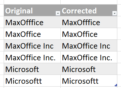
Create a table. Rename the first column as Original.
Rename the second column to Corrected.

Delete the Pivot Table. It was created just to get a list of unique Companies.

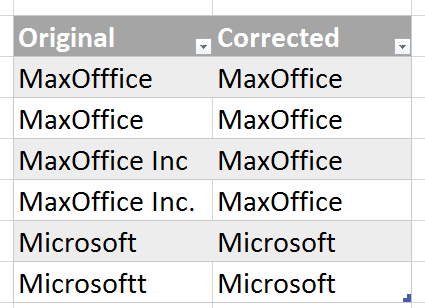
Now go through the corrected column and actually replace the erroneous data with the correct spellings.

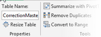
This is the Correction Master. Table Tools – Design – Change Name to CorrectionMaster

Creating this table for the first time will require effort. But for future updates, this effort is going to be reused. So it is worth putting that extra work.

Add a column in original data to get the corrected names

Go to the original data. Add a new column at the end. DO NOT add it next to the original Company column. Rename this column to Company Name (or any other suitable name)

Why not add it next to Company column? Because next month, you have to copy paste more data and that data will not have our calculated column. Simple Copy Paste will NOT be possible. If you add calculated columns at the end, incremental copy paste is very easy.
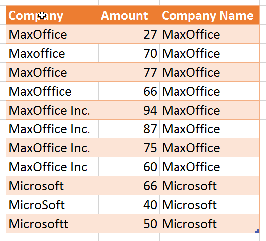
Use VLOOKUP to get the Corrected column from the CorrectionMaster

The new column will have correct names.

Create a pivot table and use the Company Name column

That’s It.

What happens when more data arrives?

Open the Incremental file. There is additional data available now.
Click anywhere (except the header row) inside the Incremental data and press Ctrl A.

The data will be selected. Now copy it and paste it below the Base file data.
The table will expand automatically.

Table will also copy the VLOOKUP formula automatically.

Notice that there are some new mistakes. Those will appear as #N/A.
Why? Because our correction master does not have entries for these new mistakes.

Filter on #N/A and copy only the Company column data.

Go to the CorrectionMaster table and copy the data at the bottom of the table.
Enter the correct names for the new entries.

Please note that when you add more data, #N/A could also represent new companies with correct names. If the workload is high, first copy paste the original column to Company Name column and then correct only the wrong names.

In-depth: I could have used an IFERROR() function with the VLOOKUP to use the original name in case the entry was not found in the CorrectionMaster. However, that will prevent you from understanding spelling variations or errors. Hence I have kept that step manual.

Go to the original Pivot Table and refresh it. You will get latest report.

Repeat this process for every update

This process has to be repeated whenever incremental data is appended and you get #N/A errors.

What Next?

We will cover the Power Pivot method of using the same concept in the next article.

Articles in this series

Grouping Text in Pivot Tables
How to correct spelling mistakes while analyzing data? (This article)
Ageing analysis in seconds (Number Grouping in Pivot)
Ageing Analysis (Numeric Grouping in Pivot) – Part 2
Ageing Analysis (Bucket Analysis) using VLOOKUP – Part 3
Grouping Dates into months, quarters and years – in seconds!
Custom Date Grouping using VLOOKUP
Grouping with Date – Time Data using Pivot

***