How to apply conditional formatting across the row

This is a common problem – which conditional formatting apparently does not solve. But that is not true. If you use FORMULA based conditional formatting, this problem has been solved decades back. Here is how you do it.

The need

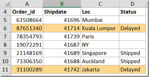
Consider this data. Status is the last column. Based upon the status we want to highlight the entire row. This is a simple example. But in real life, the data is usually spanning across multiple columns and you cannot see all columns at once.

 

Applying conditional formatting only to the status column is easy. Select the last column – Home – Conditional Formatting – Highlight Cell Rules – Equal to – Specify “Delayed”.

But this type of formatting is applied only to the status column. If status column is not visible we cannot correlate the rest of the data in that column. This requires repeated horizontal scrolling which is cumbersome.

Therefore, we need a method to apply the conditional formatting to the entire row based upon the last column value (Status column in this case).

Obvious solution does not work

You would be tempted to select the entire data and apply the above rule but it does not work at all. Why? Because when you apply any of the ready-made rules from Conditional Formatting dropdown – it is checking the value of each selected cell against the condition you specify.

So if you select all cells and choose Equal to – “Delayed”, Excel is checking if A5 is Delayed, if A6 is Delayed, if A7 is delayed and so on. Obviously, it does not work for cells other than in the status column – where the word Delayed is actually present.

How does conditional formatting work?

Conditional formatting has two parts – the condition and the formatting. Condition is essentially a formula which returns true or false. If it returns true, the formatting you specified is applied. Otherwise nothing happens for that cell.

The formula is internally copy pasted to all the cells in the selection and similar return value checking is done before deciding whether to apply formatting.

Usually this happens behind the scenes and you don’t have to worry about it.

However in this case we have to do the job ourselves because Excel is designed to compare each cell with the value you specify. If you remember, it is equivalent to Cell value contains option in older versions of Office (2003 and before).

What we need is the other option – Formula based decision to apply formatting. In this case, we will need to specify the formula.

The solution

Select all the data. Notice that the current cell is now A5.

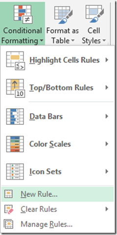
Choose Home – Conditional Formatting – New Rule

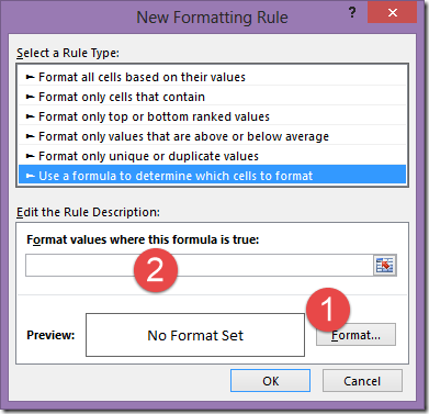
You must study this dialog carefully. This provides access to all the power of Conditional Formatting available in Excel. What we need is the last option – which incidentally is the most powerful one – Using a Formula.

Step 1 – specify what formatting is to be applied and
Step 2 – when it is to be applied.

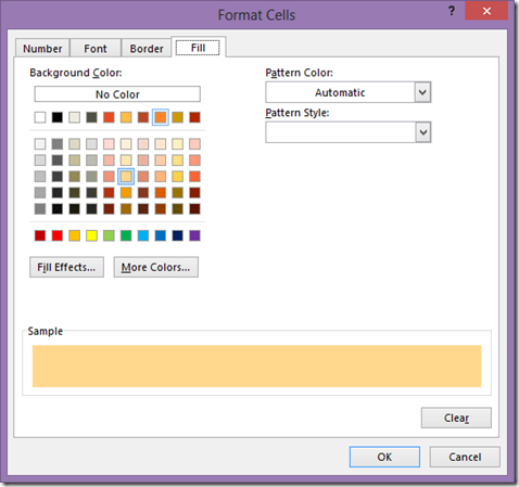
First let us select the formatting – finish the easy part. Let us choose some color to highlight delayed rows.

Be careful here. If the color has a visual meaning – for example, you want delayed rows to be shown in RED color, then choose the colors from the bottom row or from More Colors.

Why so? Because the colors on top are called Theme Colors. They can change when you copy paste this data into another Excel file containing different Theme.

Don’t know what a Theme is? No problem, read this article Understanding Office Themes.

Now the difficult part – that is to inform Excel which cells should be formatted and which ones are to be left alone.

This decision has to be taken for Each of the cells. That is why we have selected all of them. So we have to specify a formula which will be evaluated for each of the cells independently – one by one. If the formula returns TRUE, formatting will be applied.

Now, what is our condition? If the order is delayed, it should be highlighted. How do you translate that for the active cell? Remember the active cell is A5 in this case.

So which cell should be looked at to decide whether A5 is highlighted? Cell D5 – the status column. Therefore type the formula which checks if D5 is equal to “Delayed”.
The formula is:

=$D$5 = “Delayed”

Unfortunately, it does not work. Why not? Because we selected D5 by clicking in it, it automatically became a FIXED reference $D$5.
Now Excel is comparing ALL the selected cells with a single cell D5. In this case D5 is empty. So it will not apply formatting to any cell. It will not even apply the formatting to the cells which contain the word Delayed.

If you want to check, type Delayed in D5 and see. All cells will be highlighted!

Frustrating… Is it not?

But don’t worry. We just ended up confusing Excel and ourselves.

Importance of relative reference

All that we have to do is to change the formula a little.

Home – Conditional Formatting – Manage Rules – Edit the rule. Now remove the $ sign from the row number. Why? Because for row 5 we want to look at the value in D5. For row 6 we want to look at the value in D6 and so on.

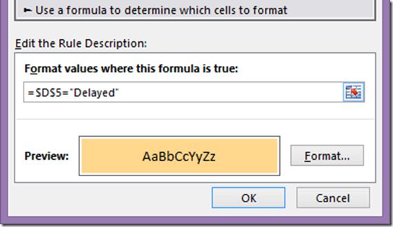
The column is fixed – Column D – which contains Status information. But the row should change dynamically. The correct formula is:

=$D5 = “Delayed”

Now try it. Problem Solved.

Change status in another row and see what happens.

Problem Solved!

Practical Notes

1. Remember to use it whenever you want to highlight a row based upon one or more column values.
2. The value need not be in the last column. It could be anywhere. Just remember to use a formula and be aware of the current cell while typing the formula. Make the row reference relative (remove $ sign from it)
3. You could also have a formula based upon values in multiple columns.
4. Nothing prevents from using a more complex function in place of the formula as long as you manage the relative reference properly.
5. In case of complex situations, it is better to type the formulas by the side of sample data – check if you are getting True False answers in the correct cells and then use it inside Conditional Formatting.
6. In this case we chose to highlight rows with Delayed shipments. If you want different color for different status items, you will need one conditional formatting formula each.
7. If you put multiple formulas make sure they do not clash with each other and that they are mutually exclusive.
8. If two formulas (which in this case means two colors) are applicable in a single row, the last formula will win. The color applied by the first formula will be over-ridden. This can lead to confusion and erroneous interpretation. Therefore, test it with large data before finalizing the rules.
9. If you use an Excel Table for the data, conditional formatting will be automatically expanded to newly added rows or columns. However, Table itself adds some visual formatting automatically. By default blue and white bands. This is a good feature otherwise. However, now we have specific color indicating a business meaning. Therefore, it is a good idea to NOT use the default table formatting.
   The simplest way to achieve that is to go to Table Tools – Design Tab – Table Styles Dropdown and choose the top left (you have to scroll up). This is called NO formatting – just plain black and white. This style does not interfere with conditional formatting but retains all the benefits of the Table.

   

 

That’s It. Do let me know your feedback by posting comments here.