Marketing: Twitter Analytics using Excel

In an earlier article, we discussed how to analyze FaceBook posts using Excel. Now let us see how Twitter data can be analyzed. This article explains how to analyze your own twitter handle data. Usage Scenarios: Product specific handles, Corporate handles, brand launches, events, live seminars, customer feedback and so on.

Steps

1. Login to your Twitter account
2. Dump the data into Excel
3. Save the file as XLSX
4. Clean up the data using Power Query
5. Load into Power View
6. Analyze

Get the data

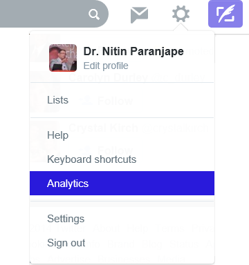
Login to your Twitter account. Choose – Settings – Analytics.

Learn what Twitter offers first

I am not going to explain native Twitter analysis here, because it is self explanatory. But explore all the items there. Even if you have gone there before, check it out again. Some new features may have been added.

By default it shows the Tweets section of analytics, as a chart and then details by each tweet.

The Followers tab shows a chart of followers along with Country, Interests and Gender distribution.

Twitter Cards provide various types of reports. The time period can be changed as desired.

Export the Tweet data

Depending upon the number of Tweets and interactions, the analysis page may take some time to open.

Now click on Export CSV button at the top.

Now choose the date range. Choose Excel format. CSV is dangerous because it is comma delimited. If there are commas in tweets, it will split those as well. Of course Power Query can solve the problem easily by splitting a column based upon the first comma instance only. However, Twitter is giving you a clean Excel file directly to you – so might as well use it.

(Of course, if the data exceeds the row limit of Excel, then you must download as CSV and import it directly into Power Query).

The file is in XLS format – Save it as XLSX, close it. Reopen it , check that all the data is available and then close the file.

The data is exported in six columns:
STATUS_ID, TIME, FAVES, RETWEETS, REPLIES, TWEET TEXT

Analyzing the data

Open a new empty Excel file. If you don’t have Power Query, download and install it. You need Excel 2010 / 2013 Professional Plus or Office 365 subscription based Office for running Power Query.

Read the article Facebook analytics using Excel 2013 Power Query:  Without programming! for details of how to use Power Query.

Click the Power Query tab and choose From File – Excel

Open the Excel file you just saved as XLSX. Now Power Query pane will open on the right side and show the Imported file and the sheet Exported Twitter Data. Nothing has been imported yet. Click on the Exported Twitter Data entry and choose Edit.

Now the Power Query window will open where we can clean up the data and import it into the data model.

The first row contains column headings.

Choose Use first row as headers option to convert it to headings.

Now, right click on the first column – Status_id and choose Remove Column. (If you want to correlate the tweets with some other data, you may want to keep this column).

The second column is called Time but actually it is date-time column. Right click on the word “time” and choose Rename – Rename it as DateTime.

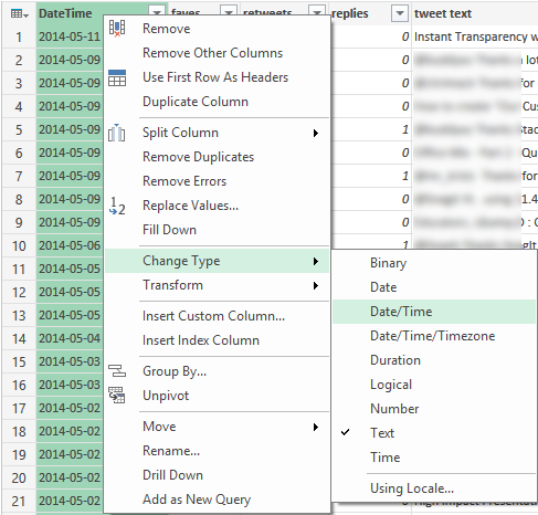
The data in the column is left aligned – that means Excel thinks it is text data type. To convert it to proper date time – right click on the DateTime column and choose Change type – Date/Time.

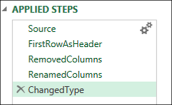
Now the date and time will be properly adjusted. Notice that the steps taken are recorded for future reuse.

By default the data will be loaded into an Excel sheet. If the data is larger than Excel row limit, or larger than say 50000 rows, it is better to choose the load to data model option and remove the load to worksheet option.

Finally click Apply and Close. Now the data will be added to a worksheet and or the data model (Power Pivot) depending upon the option you chose. I am demonstrating it using the

Analyzing the data

Let us make a simple Pivot Table and a Pivot Chart to analyze the data.

Click inside the data and choose Insert – Pivot Table. Drag DateTime into row area and Tweet Text into Value area (it will be counted automatically).

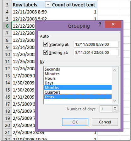
Now right click in the DateTime column and choose Group … Select Month and Year.

Now the data will be summarized by Month and Year.

Let us draw a Pivot Chart as well – Pivot Tools – Analysis – Pivot Chart – Line chart.

Right now what we are seeing is all the rows in the Tweet data.

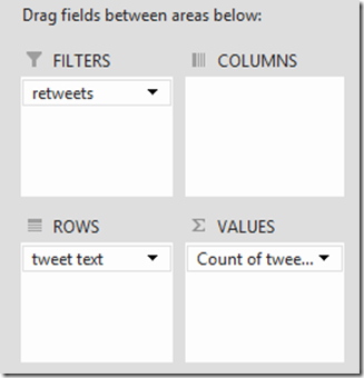
Now you can add the Favorites, Retweets or Replies fields in Filter area and refine the analysis further. For example, to know all the tweets which were re-tweeted – create this Pivot Table…

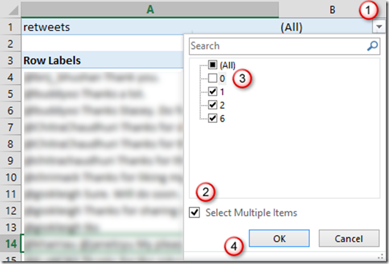
Now filter on only those items which were Re-tweeted. Open the Retweets filter drop down and do the following…

Now the data will be filtered. Similar analysis can be done on Favorites and Replies.

You can also do combined analysis by adding both to filters and see the correlation between number of Tweets which were Favorited or Retweeted in a given time period.

Hashtag analysis using Power View

Filtering on specific Hashtags is best done using Power View. Power View is available only with Excel 2013 Professional Plus edition.

Choose Insert – Power View. Now a new sheet will be added with a blank area, a filter area and a list of Power View Columns.

Drag the Favorites, Retweets and Tweet Text to the main area.

The fields will now be shown like this

The main area will show the data as a table.

But so far, we are seeing all the tweets. Not what we wanted. We want to filter by hashtags. So let us add Tweet Text field to Filter area as well.

Now it shows all tweets and allows selection checkboxes. This is not useful. Click on the Advanced Filter Mode button …

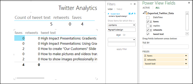
Now you get a very useful option of specifying any text which you want to look for. Here you can specify any text or #tag and perform instant search.

Here we can see the tweet text, total retweets and total favorites. But we cannot see the Total Tweets. In this case there are only few results. So it does not matter. But in case the data is large, it will matter.

So let us also create a summary table.

Create a summary card in Power View

Drag Tweet Text, Favorites and Retweets into an empty area. It will create another table similar to the one shown above. Now, in the field list area, open the dropdown of Tweet text and choose Count (Not Blank). Now, instead of showing the individual tweet text, it will just show the count.

Now you can see all three items as numeric summary. Tweets as count and Favorites & Retweets as Sums – which is exactly what we want.

This is the overall layout of what we just created.

What next

Of course there are more sophisticated tools out there. You must explore and find out what fits your requirements. The purpose of this article was to show how much you can analyze with even the most baseline data. If you use Twitter API, you can get more detailed information and analyze it.

— xxx —