Grouping is turning out to be a loooong series! But this looks like the last article in the series. How to handle date time grouping using Pivot Table. Summarize without time. Or summarize by components of time.
Estimated reading time 12 min
Potential Time Saving enormous
Please read the previous articles before you read this one:
Grouping Dates into months, quarters and years – in seconds! (This article)
Custom Date Grouping using VLOOKUP
Contents
Date and Time
Whether you like it or not, when you see a date in Excel, time is anyway available with it. If time is not explicitly specified, it is 00:00 AM or midnight. Whether you SEE the time portion or not depends upon the applied number formatting.
If you do have time portion mentioned, you may want one of the two things while analyzing it…
- You want to ignore the time portion and group by whole days OR
- You want to group by hour (or minutes or seconds)
We will explore both options.
Follow along with this sample file
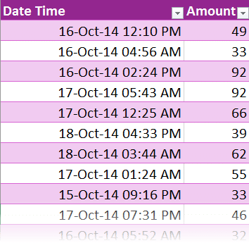
Sample Data
For simplicity we have only two columns. Date Time and Amount.
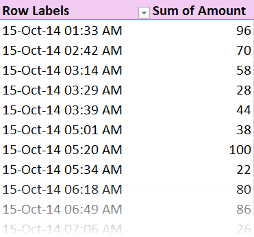
Create a pivot table. Date Time in Rows, Amount in Data area.
It does combine multiple items which have EXACTLY the same Date and Time portion. But that does not help us much. Because there still are too many entries.
If you are not interested in the time portion,
how do you get rid of it and focus only on the days?
Most of us do this by adding another column to the raw data and putting some formula. A simple formula which is INT(DateTime) will suffice. This is because the Date portion and Time portion is saved in a single decimal number like this.
17-Oct-14 12:25 AM is the same as 41929.0176
The integer portion stores the date and the decimal portion is used for time. Anyway, none of this is necessary!
Grouping by DAY while ignoring the TIME
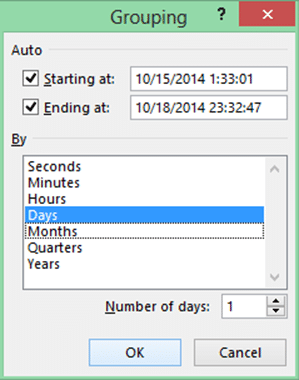
Right click in the Date Time column and choose group. Unselect Months and
just select days.
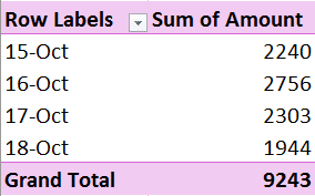
That’s it. Job done!
This is very useful in transactional data as well as server logs. Unwanted time portion can be removed in few clicks as shown here.
But the story does not end there.
Suppose we want to know how business fluctuated across time? Some hourly variation…
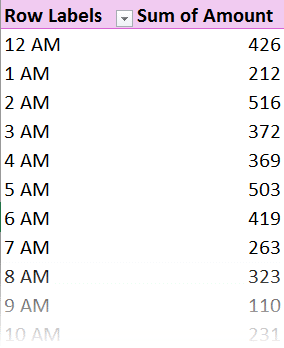
Grouping by hour
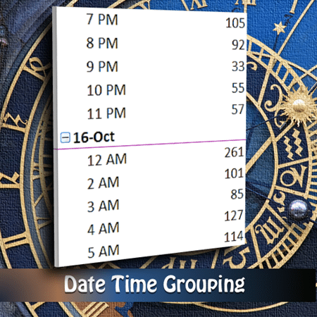
Go to the Grouping dialog, unselect Days and select Hours. That’s all.
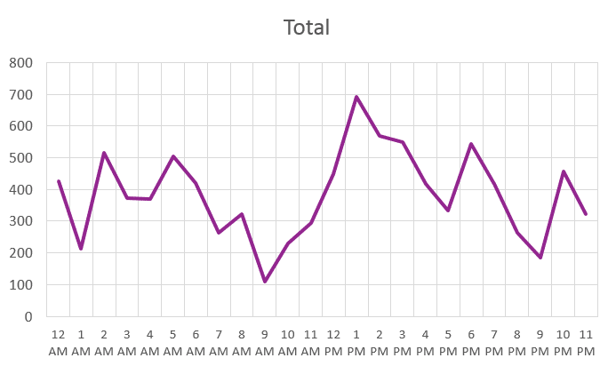
It is better to convert this to a line chart to view the fluctuation more clearly.
Vertical Gridlines make it easier to interpret the chart. Activity is higher around 2 PM.
The problem with this approach is that if we see any hour, it is a cumulative sum across multiple days. If you want to segregate each hour for each day, we need a different approach.
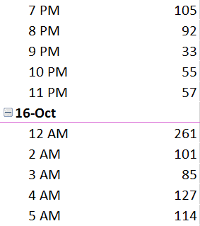
Grouping on Days and Hours
This is what you get.
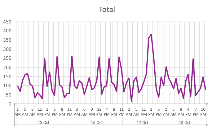
Again a line chart will show you useful information. 17 Oct around 2 PM significantly more business was done.
Working with Hours and Minutes or Minutes and Seconds
The method is exactly the same as what we did with Days and Hours. So I am not going to mention it.
Try this out with your data
The best way to learn something is to understand it first and then use it in real-life. I am sure you have understood not only the mechanics of it but also the benefit of applying it in your work.
So take some existing file (make a copy, of course) and use this approach.
Make sure you teach this to your colleagues and friends as well.
This brings us to the end of the GROUPING in Pivot Table Series.
Articles in this series
Grouping Text in Pivot Tables
How to correct spelling mistakes while analyzing data?
Ageing analysis in seconds (Number Grouping in Pivot)
Ageing Analysis (Numeric Grouping in Pivot) – Part 2
Ageing Analysis (Bucket Analysis) using VLOOKUP – Part 3
Grouping Dates into months, quarters and years – in seconds!
Custom Date Grouping using VLOOKUP
Grouping with Date – Time Data using Pivot (this article)
***

