We explore a very powerful and extremely useful approach to bin analysis using VLOOKUP.

Estimated reading time 10 min
Estimated time saving many hours (if you were doing this manually)This is a continuation article. Read this article first: Ageing Analysis (Numeric Grouping in Pivot) – Part 2
Contents
Recap
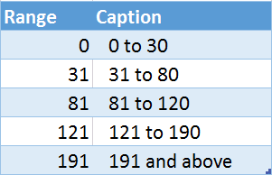
Earlier we saw how to perform bin analysis using fixed bin size. Now we will see how to manage custom bin sizes such as – 0 to 30, 31 to 80, 81 to 120, 121 to 190, above 191.
The inefficient way
Most of us will try to do such things using multiple IF statements nested into each other. Although this method works, the formula becomes very complex quickly. If you need to change the bins – you have to rewrite the formula – which is a very tricky process.
Needless to say, there is a better way.
Follow Along – use this file
The data is same as the previous file. But we have also created another table which contains the bins we require. For demo purpose, the lookup table is in the same sheet as the raw data. Usually, the lookup table will be in a separate sheet (or better still, a separate file). Keeping it in a separate file helps you in using it across reports which use similar bins.
Creating custom bins data
A bin is a range. There is a starting number and an ending number, e.g. 35 to 55.
This is a separate table. First column contains the STARTING NUMBER of the range.
The ENDING number is NEVER MENTIONED.
It is derived from the beginning of next range minus 1.

The last number of range definition is a special case because there is no next range.
It means the last number and above is the range – 191 and above in this case.
Remember to convert this data into an Excel Table.
I have also given a name (BinTable) to the table.
Put each row into the correct bin
Now we can go to the raw data and fit each amount into the appropriate bin. This is done using VLOOKUP.
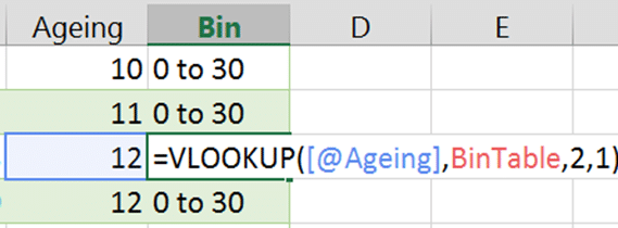
Add a new column and add a formula…

Notice that the second parameter is the BinTable table.
How does this work?
VLOOKUP looks at the value in amount and it tries to fit it into the ranges defined into the first column. When it finds the appropriate slot, it picks up the description from the second column and returns the results.
Create a pivot table for analysis
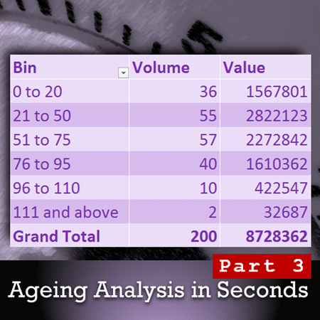
Now use this new column in pivot table to perform ageing analysis (bin analysis).

Notice that all bins are not shown – because there is no data for them. We don’t have any values for ranges from 121 to 191 and 191 or above. Therefore, those are not shown.
Changing the bins
This is not a problem at all. Just change the ranges in the BinTable table and then refresh the pivot table.

What if the data does not fit in the bins?
Our bins start with zero. There is no upper limit. So what happens if the value being looked up is below the first range beginning – say negative 4.
Now Excel has no information about what to do. Therefore it returns #N/A error.
Moral of the story: Choose the first starting range number carefully.
Power Pivot does not support grouping
Therefore, you have two choices. You use VLOOKUP on the raw data in Excel and then upload it (import it) into Power Pivot data model.
Other option is to import both tables into Power Pivot use something like VLOOKUP within the Power Pivot using DAX formula. This MSDN article by Josh Caplan explains how to do this.
Higher Learning
If you are using NESTED IF statements, it is a good idea to check if Pivot Table Grouping or VLOOKUP can help you.
Articles in this series
Grouping Text in Pivot Tables
How to correct spelling mistakes while analyzing data?
Ageing analysis in seconds (Number Grouping in Pivot)
Ageing Analysis (Numeric Grouping in Pivot) – Part 2
Ageing Analysis (Bucket Analysis) using VLOOKUP – Part 3 (this article)
Grouping Dates into months, quarters and years – in seconds!
Custom Date Grouping using VLOOKUP
Grouping with Date – Time Data using Pivot
What Next?
Now we have seen all variations of numbers based grouping.
In the next article we will explore grouping using Dates.
***


