Green mark in top left corner of Excel cells is an indication that something is wrong with the data you see. Read this article first to understand the concept: Auditors, Risk Managers, Everyone: Did you know? These green marks are WARNINGS!!
In this article, we will discuss the most important and potentially dangerous error which is commonly ignored. Read on and share it with as many people as you can.
Contents
Outdated formulas showing wrong results
This is a very dangerous and risky problem. Often un-noticed but very critical.
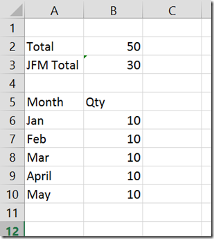
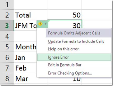
See the data. Both cells A2 and A3 are showing the green error mark. Click in cell A2, an exclamation mark icon appears. Click on the icon to display the error menu.
The error says Formula Omits Adjacent Cells. Why?
Because the formula is no including the value for May.
In this case the problem is obvious because there are only 5 rows and you can easily see that the total should have been 50. But in real life situations data can be very large and the formula results may be far away from the data. Therefore, you cannot visually cross check the accuracy of the formula. That is why the green mark is alerting you about the potential problem.
Why did this mistake happen?
Nobody wants to create formulas which omit data so obviously. The issue is that this does not happen intentionally. It happens over time. Initially data was available only for the first four months. That is the time the formula was added. Therefore the formula refers to only four cells B6: B9
After a month, more data was added and at that time someone forgot to update the formula. That is how the formula is showing potentially wrong results.
The formula is mathematically correct but operationally wrong!
These type of mistakes can happen quite often due to two reasons:
- Complexity of Excel files.
Even if you handle all your Excel files, you don’t remember which formulas are referring to which raw data. Ideally, when you add more data, you should do a Trace Precedents across the entire chain and check which formulas need to be updated. However in real life we just update the formulas we know about and remember.
Other formulas are missed out. - The second reason is Shared Files
All companies have a shared server, folder, SharePoint or some other area where departmental files are stored and used by everyone.
If someone else added a formula based upon the same data and did not inform the person who updates the data, the formula will be outdated very soon.
The operational risk of ignoring the green mark
Now you will realize the risk involved. If you ignore the green mark and assume that the number is correct, all actions which you take and all decisions you arrive at assuming that will be wrong!
Usually we do not have time to cross check every formula. It is impractical. That is why Excel is going overboard to show you the potential problem. So click on that icon and look at the available options and take the corrective action.
What is the action to be taken now?
In this case the correct action is to choose Update formula to include cells.
Now Excel will automatically change the formula to SUM (B6:B10) and the problem is solved. As there is no error now, the green mark is removed.
Alternatively you could have edited the formula yourself after checking which cells are omitted from it. Of course, this will require you to find out where the raw data is – move there, check how many extra rows were added and then edit the formula accordingly. This can be done using Trace Precedents. But the idea is, if Excel is already doing it for you, why should you bother.
Other options allow you to change the Error Checking settings (which I suggest you DO NOT change). It also provides help on the topic.
Can I select all errors and correct in one go?
This particular error DOES NOT allow you to do that. For example, if I choose both cells, B3 and B3 and try to correct both errors – you will see that the option Update Formula to Include Cells is grayed out.
Sounds unfair and tyrannical. Right? WRONG!
From the point of view of Excel, the formula in cell B3 is also showing wrong results. Because it is omitting April as well as May values.
However, what is the purpose of this formula? To calculate the total of only one quarter – Jan, Feb, March. This formula is omitting the April and May values INTENTIONALLY.
Whereas the formula in A2 was omitting cells by mistake!
This discretionary difference is only known to us humans. Excel has no way of finding out what is in our mind.
Therefore, if Excel had allowed you to correct both formulas together, the second formula would show yearly total instead of quarter total – creating another mistake.
To prevent this from happening, Excel forces you to use your discretion while choosing whether you want to update the formula or not.
That brings us to the next topic …
Should I always use Update Formula to Include Cells?
Obviously not. In case of the JFM quarter total cell – A3, we will choose Ignore Error option. Because we KNOW that this is not an error. We want it this way.
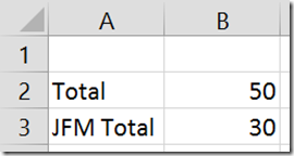
By choosing ignore error we are informing Excel that you don’t have to worry about this formula omitting further cells. Therefore, it removes the green mark from the cell.
Excel thought it was an error – You told Excel – No. It is ok with me.
In short, perform error check and then interpret
Like we saw last time, as soon as you open any Excel file, you must perform error check and take appropriate action for each cell containing and error. Once you are error free, you can trust the formula results.
Of course it does not understand logical errors or inappropriate usage of formulas. This feature is only limited to showing obvious omissions of data from the formula range.
Now my Excel workbook is error free.
Is it going to stay error free lifelong?
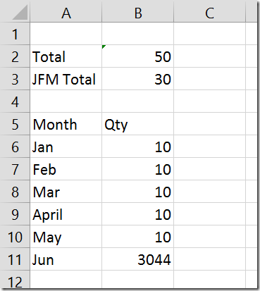
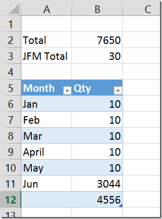
Unfortunately not. As all of us know very well, data keeps growing. In this case, next month someone is going to add another row for June value. And then what happens?
The error for A2 will reappear because the formula is again outdated – cell A11 is now omitted. However Excel is smart enough not to show error for A3 because we have already indicated that the formula is correct from a business point of view.
Again you have to go into Formulas – Error Checking – and correct all errors one by one. In this case, it is a simple demo and we know that there are no other formulas. Therefore, you can directly update the formula in B2. Now we are error free – again.
Does that mean I need to do an error check every time I add more data? That sounds very inefficient (but necessary)
In real life, the data is going to be large and complex. Formulas will be scattered across sheets. Therefore, error checking is going to take a lot of time. Performing error check ONCE is required – because we have never done it before.
However, performing the error check every time after adding data is obviously a waste of time. Unfortunately, you cannot avoid it also.
Remember what you used to do when you did not know about these green marks? You were manually going and updating all the instances of related formulas manually. Is it not?
Error checking is making that manual process at least more accurate. But the manual work is not getting eliminated.
Is there a better way?
Of course there is. Here is a recap of where we are. We have performed an error check and handled all pending errors. As of now the file is error free. And you want to keep it error free.
When you are about to add more data, you KNOW that errors will come up again and you will have to correct them one-by-one, manually. And you don’t want to do that second time onwards.
So what to do? Someone has to go and update all related formulas – but you are reluctant to do it. Then who is left? Excel of course.
If Excel is so smart that it identified this potential risk, showed me green marks, allowed me to correct the error, pointed out each error one by one to me … why can’t it become little more smart and update all the formulas automatically? Why trouble me again and again?
Very good thought. And that is exactly what Excel is capable of. But there is only ONE problem left. Excel cannot update all your dependent formulas (and references) unless you give explicit permission. Otherwise it becomes a legal issue.
You may not be explicitly aware of this, but a rule about any software is that nothing can be done without user consent. If Excel automatically updated formulas, some people may not want it / like it. Therefore, your authorization is required. Not ONCE in life. But for every block of data.
How do we authorize Excel to automatically update formulas based upon a block of data?
This is done by creating a Table. We have covered the virtues of Excel Tables earlier in these article: Excel Tables, 3 habits which highly inefficient people don’t have!!!
So here is a recap. Open a file – perform error check. Take either update or ignore action for each error. When you have an error free file, go back to the raw data – check if the data is tabular. If yes, select it and create a table.
Let us do that now. Insert Tab – Table.
For a table to be created, the data must be in columns and each column must have a unique heading. No empty headings. No merged cells. No empty headings. If all this is alright, click Ok. Refer to the article Good Data vs. Bad Data: How to identify? for details.
Now the data becomes a table. It is automatically formatted and you see a new tab called Table tools on top. If you see this tab, it means your current cell is inside a table.
The small dark blue marker at the bottom right corner can be used to drag and resize the table in case you missed some rows or columns while creating the Table.
Now if you add more data below Jun, it is Excel’s responsibility to update all the formulas and references (all dependents). You don’t have to remember to update formulas, neither do you have to perform repeated error checking and correction.
Formula updates for that block of data have now become AUTOMATIC.
Formulas, Pivot Tables, Data Validation Ranges, Vlookup Formulas, Named Ranges, etc. which depend upon this range will all have been updated by Excel immediately and automatically. This works across sheets.
In fact, if there is a file linked to this data and if that file is open, Excel will update those references as well. However, if the file is not open, Excel is helpless and cannot update those references. This does leave a lacuna which you need to manage manually by remembering to open linked files before updating related data.
Unfortunately, it is easier said than done. Because in a typical company, there are so many files linked to each other – without any formal documentation – that it is practically impossible to be 100% certain of anything!
Tools which find dependencies work from the dependent to independent side and not other way around. Therefore, this particular issue remains unsolved as of now. There is a new server based tool which is called Discovery and Risk Assessment Server – a Microsoft product which works on top of SharePoint server. We will cover it in a future article.
What if my raw data is not tabular and
therefore I cannot create a table?
In this case, you will need to maintain the formula updates manually. Before you add more data, you will have to click on an existing data cell and use Trace Dependents from Formula tab to find out all the dependents and update them manually. No other choice.
It may be a good idea to revisit the structure of your non-tabular data and see if it can be converted into tabular data (we call it Good Data). In many cases, I have observed that this is possible – and it leads to phenomenal improvement in efficiency as well as accuracy.
Benefits of this approach
Using Error Checking and Tables we got dual benefits.
Time saving
This is the obvious benefit. Because you are no longer going to waste time manually updating formulas or correct errors.
Increased Accuracy
Although this is an intangible benefit, this is the more important part. Accuracy is absolutely necessary for business sustenance and earlier we did not even know the level of inaccuracies entrenched into your organization!
Recommended Best Practice
Progress Tracking
There are 9 types of errors which are indicated by the green mark. We just finished ONE of them. We will cover more in future articles.
Who should know this? Everyone!
Every user of Excel should know this. Please share this with everyone around you. Make this a standard operating procedure for Excel across your organization.
How? Just refer everyone to this article. Plead with them to spend 20 minutes reading this and the previous article. Everyone will benefit. Trust me.
If you have any queries, do post them here. Your feedback is also welcome.
***


