Data Split into Two rows – Cleanup using Power Query

This is the worst type of input data to get. Each row has been split into two (or sometimes more) rows. We want those to be combined into a single row. In an earlier article, I have shown one method of doing this.

Now here is a simpler, faster and more powerful method using Power Query.
(Estimated reading time 12 min)

The Data

Download the Zip file containing two sample files – Raw data and Merged Data. Start with the Raw data file and follow the steps.

Data is actually supposed to be shown in a single row with many columns. But it has been split into two rows. The blue part is first row and red part is second row. Even the header is split into two rows.

The objective is to create simplified version of the data where the Customer Type, Segment, Listed and Type of Sale columns are adjacent to the Ageing column and there are only 6 rows of data (instead of the split 12 rows).

The Logic

Before we see the actual steps, understand the concept.

1. We do it in three steps.
2. In the first step we gather all even rows, second step gather all odd rows
3. In the third step we combine them together

Now let us translate this concept into reality.

Cleanup using Power Query

1. Notice that the data is already a table. If not convert it to a table. The last column name (Column1) will be added forcibly when table is created. Do not worry about it.
2. Now go to Power Query – From Excel Table and select the data
3. Power Query window opens. Now check if the first row is being considered as the header or not. If not, choose Use First Row as Headers.

   

4. Remove the unwanted Column 1. Right click on header, Remove Column.
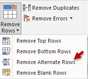
5. Now we want to get rid of alternate rows. Choose Remove Rows – Remove Alternate Rows option.

   

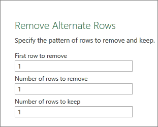
6. This is a very powerful, but confusing option. Read the dialog carefully before filling in the values.
   In this case we want to get rid of the 1st, 3rd, 5th, …. rows. That is why the following values are needed.

   

7. Now the unwanted wrapped around rows and their header is gone.

   

8. Remove the last Column1
9. We need a new column which just provides a unique id for each row – like a serial number. This is called an Index Column. Open the Table menu and choose Add Index Column – Starting at 1. This is what happens…
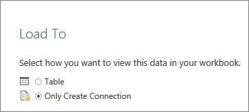
10. Now we will just save the query. Name it as LeftSide. Close and Load to, Create Only Connection.

    

11. The query will be shown as saved in the Queries Pane.

    

The first step is done. Now let us create a query for the second rows of the data.

1. Go to Power Query and choose From Table and choose the same table.
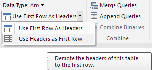
2. This time we want to get rid of the odd rows. If the first row is already taken up as the header, we want to undo that. Choose the dropdown of Use First Row as Header and choose Use Headers as First Row. It is a confusingly named option. It basically means, demote the first row if it has been considered as a header.

   

3. Now the data looks like this. We want to get rid of the 1st, 3rd, 5th, … rows again.

   

4. Therefore, we follow the same steps again. Remove Rows – Remove Alternate rows, All parameters 1, 1, 1. Click OK. Now we have the Odd rows remaining, including the header.

   

5. Now promote the first row as header and remove the unwanted Column.
6. Remove the unwanted Column1
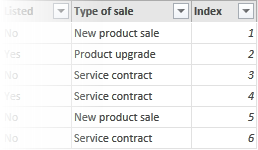
7. Add an index column here as well – starting at 1

   

8. Save this query as RightSide (Create Connection Only).
9. Now both queries are shown in the workbook queries pane.

   

The next step is to Merge both the tables (queries)

1. Right click on the LeftSide query and choose Merge
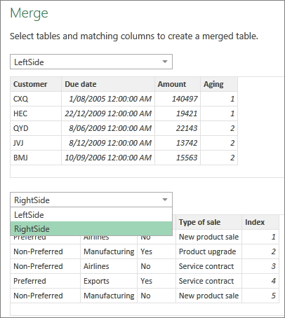
   A dialog appears showing the first table.
   Choose RightSide from the drop down in the lower half.
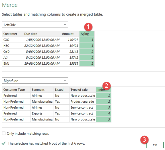
   Both tables are shown.

   

2. Now click on the Index Column on both tables and choose Merge

   

3. Now the tables will be shown as combined, but the second table is not shown fully. It is shown as a Table hyperlink.

   

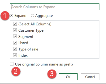
4. We need to expand that table into its actual columns. That is done by clicking on the double headed arrow next to NewColumn

   

   Clear the checkbox Use Original …

5. We are almost there now. Remove the unwanted Index columns now.

   

6. Now choose Close and Load To and decide whether you want the combined table to be dumped into an Excel sheet or Power Pivot Data Model.
7. Save the file. If you don’t want the original data to be connected to the queries, go to each query and use Unlink option from the query tab. Once both queries are unlinked, you can delete the raw data, the queries themselves and keep just the combined tabular final version of the data.

I know it sounds a bit complex. But try it out couple of times and you will learn it quite quickly. Of course, if you have three or more rows spillovers, the same concept applies. Just tweak the Remove Alternate Rows dialog and create three queries, add index columns to them and merge them.

Enjoy!