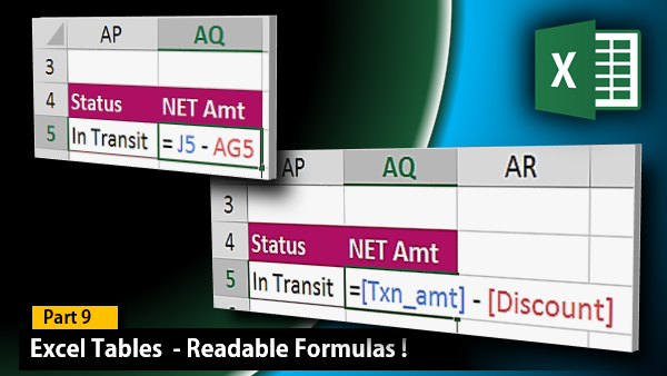
Readable formulas in Excel tables are so nice, you will curse yourself for not noticing earlier (since 8 years!). Teach this to everyone around you – NOW! Show off ![]()

Contents
Calculated Columns
We get raw data from reports or database dumps or text files. We often need to add more columns which are based upon some calculations on top of the raw data columns. These require a formula to be added and copied all the way down.
We have seen in the earlier article that formula added gets auto-copied by Table.
Now let us go one step further. Here is a simple calculated column showing NET amount.

This is a very common activity. But imaging the pain involved if there were 78 columns in the data and you wanted the NET column to be in the 79th column. You would have to press Left Arrow repeatedly 78 times to reach the amount column. And repeat that 77 times to reach the discount column. (Obviously we don’t remember which data column is in which Excel column).
The new way – Readable formulas
Now consider this. I am typing this formula the traditional way. Type = sign and press left arrow twice to reach the AMOUNT column. And see what happens…
You would expect Excel to show you C5 but it shows something unimaginable but surprisingly simpler.
You continue to type the formula as usual, type the minus sign and again press Left Arrow to move to the DISCOUNT column…
And of course, when you press ENTER, the formula gets copied automatically. That is why I typed it in the second row – in fact it does not matter which row you type the formula in!
Benefits
You no longer have to struggle pressing LEFT ARROW many times searching for desired columns.
The formula is much easier to understand. You yourself are going to forget the exact calculation after a few days. So if you (or someone else) looks at a formula which says …
= B9- AK9
You have absolutely no clue about what the formula is calculating.
Instead of it if you see…
= [@Qty_sold] * [@Unit_price] – [@discnt]
you will understand it much better. Not just you – everyone else as well. All thanks to the miraculous Excel Tables.
If the columns are far away…
Think about it.. you are in the 79th column and you want to use the new syntax with Column Names in the formula. But you don’t remember exact column names. It is not practical to do so. Now what?
In order to find the exact spelling of each column name, you will still have to navigate manually to some far away column. So where is the efficiency increasing? Same effort like before.
But wait, don’t we know that the column names can be used as long as they are enclosed in square brackets? So let us put a square bracket to start the process and see the magic…
Excel knows that you will face this problem – and it solves it elegantly. It shows a list of all columns in the table. Now you just type the first few characters to reach the desired column and press TAB to make Excel type the full name. You must close the bracket manually.
The meaning of @
We will cover this in greater detail later. But for now, @ along with field name means take the value from that column for current row only. If you remove the @ sign, the entire column will be referred to.
The syntax is more complex in 2007. But simplified from 2010 onwards. In any case, when you are learning, let Excel type the syntax automatically. In 2007, instead of @, it used [#THIS ROW].
What Next
In the next article, we will see the MOST IMPORTANT and ULTRA-SOPHISTICATED feature of Tables. Automatic dependents update. The world will be a better place if everyone uses this! Unfortunately – not many people do
Related Articles
This article is a part of the series: Knowledge Pack – Excel Tables
***


2 Responses
This field reference is very useful !!
Reblogged this on SutoCom Solutions.