Combine Multiple Sheets into One Sheet

The query keeps cropping up very often while I work with customers. There are many ways to handle it. Here are three ways to do it. Simple Copy Paste, using VBA and using Power Query.

Exact Requirement

You can follow this article with a sample file.

Input

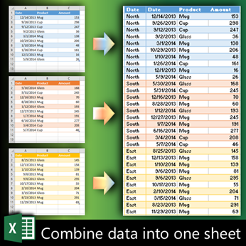
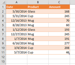
• There are multiple sheets containing tabular data. (4 sheets, 10 rows)
• These may be in the same workbook or different workbooks.
• Each sheet contains the same columns in the same order
• Each sheet represents some property or source
  Usually it is month, region, location, person, product, etc..

     

Output

This article does not cover cross-tab data. Please read these two articles for consolidating cross-tab data.
Consolidating crosstab data
Crosstab data consolidation using Power Query

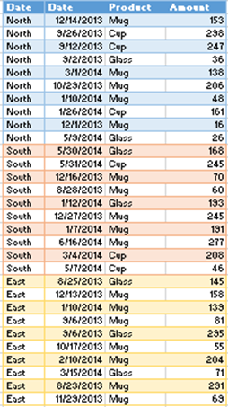
Now what is expected? Most people just want to combine all the data across sheets into a final sheet which contains all 40 rows.

Please note that we are not interested in performing any summary calculation. This would typically done using Pivot Table / PowerPivot or Power View AFTER the data is combined.

Now when we combine the data from all regions into a master sheet, the data got mixed up. Therefore, while combining data from multiple sheets into a single master sheet, the individual sheet identity must be preserved. This is done by adding a new column to describe the additional information.

With this in mind let us see various approaches available to us.

The logic

1. Create master sheet (or separate file)
2. Copy first block of data including the header row
3. Paste it into master sheet
4. Convert it to a table (Ctrl T)
5. Add a new column (ideally as the first column) to identify the original sheet context (in this case Region)
6. Copy the identity to all rows of the first block
7. From second sheet onwards
   1. Copy the data from the sheet WITHOUT the header row
   2. Paste it below the last row in the master sheet
   3. Copy the identify of the sheet to all the added rows

This logic has to be used irrespective of which method you choose.

Simple, manual copy paste

This is easy and probably the best way if you have very few sheets to combine and the data is not large.  The logic above has to be manually implemented.

Office Clipboard

The manual approach requires multiple operations of COPY and PASTE

This is a brilliant but unknown feature which gives you 24 clipboards.
This way you can do COPY, COPY, COPY, COPY and then one single PASTE ALL

To understand how this is done, read these two articles…
Copy Paste – Part 10 – How to get 24 clipboards
Copy Paste – Part 11 – Why do we need 24 clipboards?

The disadvantage of this approach is that during the Paste All operation, you lose the source identity of each block because all blocks are pasted at once.

The solution is to include the header in each copy operation and remember the copy order. After Paste All you can identify each block by repeating header and then add the source identifier data. Finally you will need to remove the repeated header.

Use Third Party Tools

Here are some popular utilities for Excel which provide this functionality.

http://www.ablebits.com/excel-add-ins.php
http://asap-utilities.com/
http://www.extendoffice.com/product/kutools-for-excel.html

Use VBA

The code is fairly simple. But I am neither going to give you the code here nor point you to another site. Why? Because the exact positioning of the data on the sheets and the layout is so varied, that unless you have a good user interface to handle variations, simplistic VBA code is not going to work. The tools shown above do a good job. So use it.

If you want to do it yourself, use the logic above and write the code.

Power Query

This is a new approach where we can use the Power Query Append feature. To use Power Query you must have Office 2010 or above – Professional Plus version. You can download Power Query from here.

The steps are as follows.

Convert Raw data to table

Power Query imports data from a table therefore convert each raw data into a table. This is easily done with Insert – Table or Ctrl T.  Open Table Tools tab on top and change the name of each table to avoid confusion later. Ideally the source (sheet name) should be used to identify the table.

In this case I have four tables called North, South, East and West – same as the sheet names. In some cases, the sheets may not have specific names. You must still use good and legible names for each table.

Create queries for each sheet but DO NOT import data yet

We will create four queries – one for each input table and add the source identifier column to it. This is done by creating ONE query and then duplicating and modifying it.

Create first query

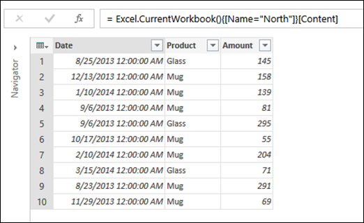
Click inside one of the tables – in this case North and choose Power Query Tab – From Table.

Edit the query

The query editor opens. The name of the query is automatically set to “North”. Data from North table is shown.

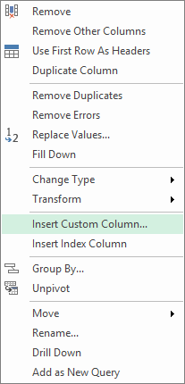
Right click on any column heading and choose Insert New Column

New Column dialog opens. Add the text “North” manually and click Ok.

This adds the column with each row containing the text North.

Now the query is complete. But we do not want to load data as yet. Therefore, clear the checkboxes as shown in the Load section. We just created a query definition. We will use it later.

Now choose Home – Apply and Close to return the the Excel workbook.

Now a window (pane) will open on the right side showing workbook queries. The North query will be visible. We have four tables with similar data. So we will duplicate the North query three times. Right click and choose Duplicate. Create three duplicates.

   

Modify the queries to get data from all four tables

Edit the North (2) query. Change the name to South. Query Editor shows the steps on the right side. Click on the Source step.

In the formula bar – change the source table name to SOUTH.

Click on the second step – where we added a new column. Change the content of the column to South.

Save the query. Do these changes for the remaining two queries as well (East and West).

You can also make changes quicker by choosing Advanced Editor in the View tab of Power Query

Append the queries

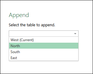
Open the last query (West query in this case) in Query editor. Choose Append Queries from Home tab.

Choose another query to append to the West query and click Ok. Repeat this process for South and East as well.

All the data is now combined in the last query. Change the name of the query to something like “All Data”. The final code in Advanced Editor will be like this…

Load the data

Now you can choose where you want to load the data. If data is small, you can use worksheet. Otherwise load it to the data model.  Now you are ready to perform further analysis.

Query written directly using M language in Power Query

Finally you can create a new blank query and use the syntax above to create a parameterized script in M language. Here you define an array containing the list of tables and iterate through it to perform the activities we earlier did manually.

Importing into a blank spreadsheet

In this demo we chose the same file for Input data and the combined data. In real-life, if the data is very large, it is better to create a new blank file and use Power Query to import data from another Excel file which contains the original sheets. This way, there is no duplication of data in the current file – thus improving performance.

Remember that if you import data into a blank workbook by connecting to another workbook, you cannot import tables. You must select each sheet.

Benefits

This methods sounds much more cumbersome than manual copy paste! In reality, the Power Query method is very powerful and scalable. If the data is large, the manual copy paste approach will simply not work.

Another benefit of Power Query is that if the data source is changed, you can just refresh the data instantly without having to do any other manual work. This would be impossible to achieve with manual copy paste.

Another benefit is that the additional column is added automatically by Power Query. In case of manual method, you will end up spending lot of time copy pasting the region names (source identifier).