Creating Table of Contents for YouTube Videos

If you post a long video to YouTube, it is a good idea to add a Table of Contents to the description. This helps viewers go to specific topics quickly. In my case, I post the video link + TOC on my blog as well. The link format for YouTube and regular HTML are totally different. That is why I made an Excel based YouTube TOC creator.

YouTube TOC Creator Usage

1. 1. Upload your video to YouTube
   2. Copy the Sharing link for the video from YouTube:
      It looks like this :

• Download the Excel file YouTube TOC Creator V3.xlsx
• Paste the link in the cell B2
• Overwrite the Sample row with your data
• In the first column specify the Topic name
• In the next 3 columns specify the Hour, Min, Sec for the point where the topic begins. All three must be integer numbers.
• Hours can be 0 to 12 and minutes / seconds can be 0 to 59.
  DO NOT enter the unit. For example if you are entering 12 minutes, just type 12 in the Minutes column. Do not type 12 min
• Add multiple topics and start time as required
• Now you get three types of Table of Contents

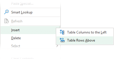
The TOC data is in an Excel Table. I have provided 35 rows. If you want more rows, right click inside the table and choose Insert – Rows above.

If you type the topic and time data outside the table, formulas will not be calculated.

Types of Table of Contents

1. Just URLs (green column)
   The URL requires time converted to seconds. This is done automatically for you.
2. YouTube Description data (yellow column)
   In YouTube description, you just need to type the topic followed by the start time in hh:mm:ss format. This is automatically created.
3. HTML Links (red column)
   In case you want a proper HTML <a href> tag – typically for embedding in a web page, use the red column.

Choose the desired rows from the required column and paste the data to the desired location. That’s it.

I hope you find it useful. If you have any ideas for enhancing the YouTube TOC Creator, let me know (post comments).