This is a very old feature. But it is still very useful. Spend 10 minutes to learn where you should use and not use Range Names in Excel.

The Need for using Range Names in Excel

Often we use the same cell in many formulas. For example, tax rate, discount percentage, constants (like Pi) and so on. Every time, we have to refer to the sheet and cell address. This makes it difficult to type, read and understand the formulas. Instead of referring to a cell using the sheet name and cell address, we can refer to it using a more legible and easy to understand name. That is called a Range Name.

How to create Range Names in Excel?

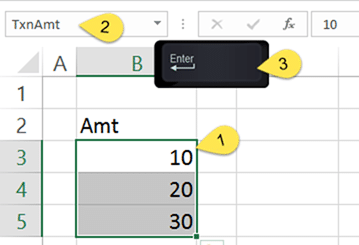
The simplest way is to select the cell or cells and type the name in the Name Box. Where is the name box? It is on the left side of the Formula bar.

Just type the name and press Enter key. That’s all.

The name must start with a character and cannot contain spaces.

Of course, it should not clash with any cell name (e.g. RUN4)

Another way to create names is to go to Formulas tab – Name Manager and choose New. By default, all names must be unique across sheets (at workbook level). If you choose Sheet in step 2 below, then the same name can repeat across sheets.

How to use Range Names in Excel?

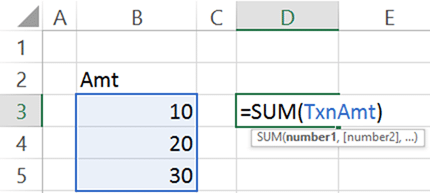
Once created, range names can be used in any formula, instead of the actual reference to the range itself.

What if we need to create lots of names?

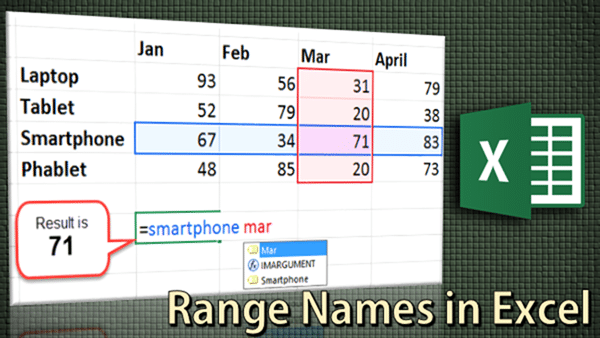
Consider the data below. There are names for each column and each row. This type of data is called a cross-tab. Creating so many names manually will take a long time. Moreover, the name which we intend to use for each of the ranges, is already written as a row and column heading.

In such cases, we can ask Excel to do the hard work and create names automatically. Choose Formulas – Defined Names group – Create from Selection (which means Create Names from Selection). Choose Top Row and Left Column in this case.

Now all the names are automatically created. You can see all the names by opening the dropdown next to the Name Box.

The benefit in terms of time saving is obvious. But that is not all. Now that the names are created for each row and column, we can use it to get the cross-sectional value.

Finding the value at the intersection of specific row and column using Names

Look at the data again. Suppose I want to find out the value for Smartphones in Mar. That value is 71. Usually we use Index and Match function combination (or Vlookup / Hlookup) in this case.

Now, we have a much simpler method available. Just type a formula (starting with the equal to sign, as usual) containing the row name and the column name separated by a space. That’s it. The formula will give you the desired value of 71.

Issues with range names

In the data above, the name Jan is currently including four rows. Suppose we add another value for Jan below the number 48, the defined name will NOT understand it. We have to go to name manager and manually make the change. But if you use Excel Tables, this happens automatically. When data is added, Excel table will automatically extend the range name. This works only in the vertical direction (not horizontal).

Of course, there are many more practical uses of Range Names in Excel. But we will cover those in later posts.