We continue to explore Pivot Table Grouping. This time we work with grouping dates. If you do this manually, the method shown here is like a miracle for you.
Estimated reading time 10 min
Potential time saving many hours
Contents
The Need
All transactional data usually has a date column. In fact you may have multiple dates like order date, shipping date, delivery date and so on. Usually, Time is also captured along with dates.
We often need to summarize daily data into weekly, monthly, quarterly and yearly reports. Typically most of us add more columns next to the original date column and use various type of date time functions to get what we want. STOP doing this manually.
Pivot Table provides you with an INSTANT solution for this purpose.
Download file and follow along
There are two sheets. Both seem to have the same data, but there is a difference.
The earliest date we have is 28 Feb 2013 and latest date in the data is 16 Oct 2014.
Grouping dates
Go to Sheet1. Click inside the data and create a Pivot Table.
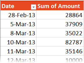
Drag DATE to row area and AMOUNT to value area.
Now right click inside the date column and choose Group…
You should get an error message.
Why did this happen? Go to sheet1 and scroll the data. Did you find the problem?
Some dates are blank. Some dates are not being recognized as dates (Left aligned dates are text).
If you don’t consistent data, this feature does not work. Therefore you must check the data before analyzing. You can do this checking using Pivot Table itself. Read this article for details: New use of Pivot Table – Data Quality Audit
Delete the Pivot table you just created.
Go to Sheet2. Here the dates are consistent. Create a Pivot – Date into rows, Amount into Values.
Right click inside the date column and choose Group… option.
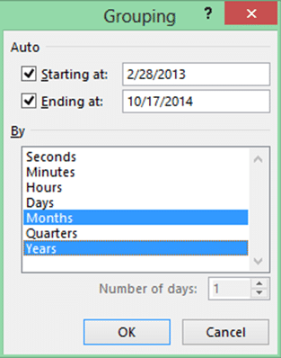
This dialog is where the magic happens.
All the units of summary you will ever require are here.
The list is also special – it is a auto-multi-select list. There is no need to CTRL-CLICK to select multiple options. Just click is enough. By default it is in multi-select mode!
Months is already selected. Just click on Years also. Then click Ok. That’s it.
Grouping only by months
Go to grouping dialog and remove YEAR option. Now all months across years are combined. This is useful if you want to see if there is any seasonal variation in the data.
Grouping by Quarters
If your financial year starts in Jan – this is a very useful option for you.
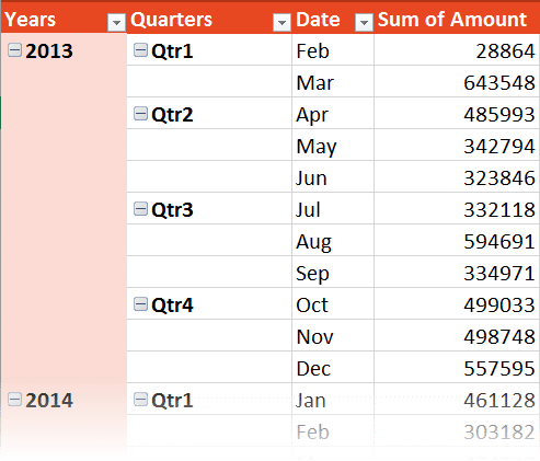
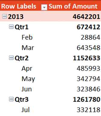
Now choose Month, Quarter and Year. See the results.
Notice that each level of grouping is occupying one physical column. It also leaves blanks for the subcategories. To avoid this wastage of space, go to Pivot Table Tools – Design – Report Layout – Show in Compact Mode. Also choose Subtotals – Show totals at the top of the group. Now it occupies only one column and saves on space horizontally as well as vertically.
If your financial year starts in any other month, this option is of no use to you. (We will cover the solution for this issue in the next article). Calculated Items option does not work if you have used Grouping.
Grouping by weeks
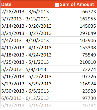
Choose Days and unselect all other items (Month, Quarter, Year). Now in the textbox below, type 7. It now groups by days.
This is good. But the week may not start with the day of your choice. It will start from the day of the earliest date in your data. This may be a Tuesday or Thursday or any other day.
If you want to ensure that the grouping starts from, say Monday, you must change the starting date.
Enhancing the analysis
Remember to use all the Show Values As options to gain more understanding about the data. Also remember to apply relevant conditional formatting to simplify interpretation.
Customization Required
Sometimes the months may not end on the last day of the month. Sales may continue for few more days and the finish the monthly processing by 2nd or 3rd of the month. There is no way to handle this in Pivot Table.
Similarly, as mentioned earlier, financial years which start with any month other than 2003 require different approach for calculations of years and quarters.
Both these problems can be solved using VLOOKUP based additional column in the raw data.
Power Pivot Solution
Power Pivot really shines in this aspect. It does not have the Grouping option, but it does offer complete flexibility without any manual work.
In brief, you create a separate table which contains all the dates across years into a single column. Add more columns for various summary parameters like Year, Month, Quarter, Weeks, Holidays, Working days and so on. After importing the table into Power Pivot, you create a relationship between your raw data and the TIME table.
Once this is done, any kind of grouping can be managed very easily.
More importantly, PowerPivot language (DAX) provides extremely powerful functions for time period based calculations like cumulative summary, comparison with pervious years and so on. We will explore Power Pivot in a separate series of articles.
Articles in this series
Grouping Text in Pivot Tables
How to correct spelling mistakes while analyzing data?
Ageing analysis in seconds (Number Grouping in Pivot)
Ageing Analysis (Numeric Grouping in Pivot) – Part 2
Ageing Analysis (Bucket Analysis) using VLOOKUP – Part 3
Grouping Dates into months, quarters and years – in seconds! (this article)
Custom Date Grouping using VLOOKUP
Grouping with Date – Time Data using Pivot
What next?
We will explore custom quarters and custom months using VLOOKUP in the next article.
***






2 Responses
Very useful article! Thanks, Doc!
Thanks Vinay. See the whole pack of 51 articles called “Knowledge Pack: Data Analytics“. You will find it very useful. Share it with your team as well.