Before you perform manual calculation, learn this option. This can save you hours of manual work. Estimated reading time 10 min

This article can be read independently, but it is a part of the series which covers a bigger problem of trying to add formulas OUTSIDE the pivot table manually. Please read these articles to understand the full context:
Adding formulas OUTSIDE Pivot Tables = Inefficiency
Pivot Table – Show Values As – Part 2
Pivot : Show Values As – Part 3
Pivot: Running Totals and Ranking
Contents
Download Sample File
Download this sample file
This file contains simple raw data. Each row is a transaction.
Some terminology you must know
Regular Pivot Table is created from ONE block of data which contains rows and columns. Each column has a name and consistent data.
Each column is called a FIELD.
Individual data contained in a column are called ITEMS.
For example, in our sample file…
Year, Month, Amount, Discount are FIELDS.
Jan, Feb, Mar, Apr are ITEMS in the FIELD called Month.
Similarly 124, 154, 126, etc. are ITEMS in the field called Discount. But there are too many different items. So in practice they are less relevant – as you will soon see.
Each FIELD has a SINGLE type of data in it.
For example, Amount and Discount fields contain numeric data.
Month field contains text data.
Numeric fields are used to create additional calculations – for example, we could add a NET amount column with the formula Amount minus Discount. But we don’t want to add that NET amount column in the raw data. Why not add it to Pivot Table itself?
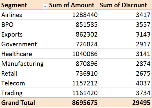
Base Pivot Table
Rows: Segment, Data: Amount and Discount.
Now we want to calculate NET amount – which is a simple subtraction operation.
It is VERY TEMPTING to add a formula manually in the adjacent column. But resist that urge. That would be like “You helping Excel” which is inefficient.
Let us ask Excel to help us.
Calculations using one or more fields
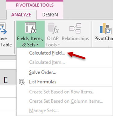
Click inside the data area. Choose Pivot Table Tools – Analyze Tab – Fields, Items and Sets dropdown – Calculated Fields…
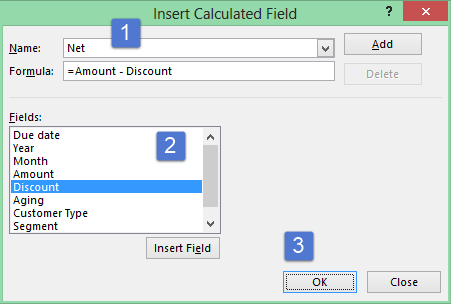
Now you can add a formula here and give it a name. We will call it Net Amount and specify the simple formula. Amount – Discount
Please note the order. Just type the new name for the field.
DO NOT delete the = 0 formula.
Just double click on the Amount in the list.
Then type the – (minus) sign and again double click on the Discount.
Why is this double click important?
Because this place has its own special syntax. Which you don’t want to learn.
For example, if you added the Customer Type field, because it has a space in its name, it has to be enclosed in single inverted commas as shown below. You will not know this and you will get an error. To prevent this from happening, always double click on Field (and Item) names while adding formulas.
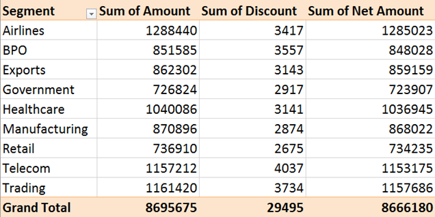
Anyway, now the job is done by Pivot Table itself.
This Net Amount field is also added to the field list…
Remember: This is a calculated field. So it can only go into Data area. You cannot put it in Row, Column or Filter area.
Also remember that it like any other calculation in data area. So ALL the options which we just saw with Show Values As will work on this field as well.
Only want to show Net Amount?
Remove Amount and Discount
This calculation is being done internally by Pivot. It does not need both the original columns to be visible. Remove them. It will still show the NET AMOUNT.
To go one step further, if you add something in column area or row area – it will continue to calculate NET AMOUNT in each context.
Compare this with what you would be doing if NET was calculated manually. Pivot is not just doing the simple calculation for you – it is making it completely dynamic and flexible.
It is not just a faster substitute – it is giving you an unbelievable (but very useful) capability.
Multiple calculated fields
Once you create a field, you can use it for further calculation to create
more calculated field(s).
One constraint. You cannot use an external reference cell in these formulas. You will need to hard code the value 3. You cannot refer to some cell which contains that value.
Document the formulas in one click
Choose the List Formulas option. A new sheet is added with details of each calculated field and the associated formula.
Use it with your data and tell this to everyone
For all you know, your colleagues, friends and family may be wasting their precious life trying to do such things manually. Tell them about these great features immediately.
What Next
We will see how to create calculations using ITEMs in the next article.
Articles in this series
Adding formulas OUTSIDE Pivot Tables = Inefficiency
Pivot Table – Show Values As – Part 2
Pivot : Show Values As – Part 3
Pivot: Running Totals and Ranking
Adding calculations WITHIN Pivot Tables (this article)
The amazing Calculated Items in Pivot Tables
***





One Response
Thanks for the good article.
Can you please elaborate on the limitations of Calculated Fields / Calculated Items in one of your blogs.
I am trying to use ‘Group’ function on a value field (for which I have already added a calculated Item in another pivot table). Even though I am trying to use the ‘Group’ function in a separate Pivot Table, excel somehow finds out that as source data is same for both pivots.
The same problems happens vise versa as well. i.e. after I use the ‘Group’ function on source data and then create another pivot table where I want to add ‘Calculated Items’, Excel throws error ‘You can not add Calculated Item to a grouped field’.
Also, Calculated Field does not return correct value if I have used ‘Group’ function in a Pivot table.
It will be helpful if you can write a blog on correct sequence of using ‘Group’ funcion, ‘Calculated Items’ and ‘Calculated Field’.
Regards,
Amulya