In this article we will learn the actual steps of delivering Excel reports: Create a report in Excel, Publish it in SharePoint and Share it with others. Please read the previous article before reading this article.

Estimated reading time 10 min
Contents
Pre-requisites
Excel 2013, SharePoint 2013 (Enterprise edition) or Office 365 with SharePoint. Some of the functionality will work with SharePoint 2010 as well.
The process
Here is what we want to do … same diagram from the previous article.
Get the data and Create the reports
I am not going to spend time on how to create reports. For the time being, let us assume that you have already created the summarized reports in the form of Power View Sheets, Pivot Tables and Charts. You may also have some manually created custom reports on specific sheets.
Decide what you want to display as a report
Ideally we don’t want to show all the contents. Most of the content will be raw data, intermediate calculation or supporting worksheets. Usually only the final report, which you usually copy paste as values into another file – is what we want to show.
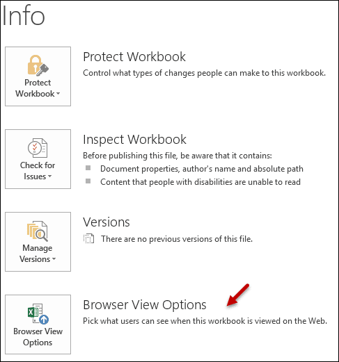
This is done using File – Info – Browser View Options.
By default all the sheets are shown. Choose the required option and save to SharePoint site.
However, you can choose the sheets you want to display.
Showing entire sheets is a good idea for custom reports which are manually created. It is also the only option available for Power View reports.
Now only the selected sheets will be shown on the browser on SharePoint site.
This approach has one disadvantage. The report components like pivots and charts may be scattered across the selected sheet. They may not be visible without scrolling. Therefore, it is a bit cumbersome to discover all components of a report – especially if these are lying on multiple sheets.
Therefore, the third option was provided. This is the most powerful option.
Items in the workbook
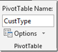
Every pivot table, table or chart can have a name. Default names are like Table33, PivotTable2, Chart19 and so on. But you can change the names.
Change Table name from Table tools – Design menu, Pivot table and Chart names from Analyze menu.
Choose the items you want and then save the file to SharePoint or OneDrive for Business.
Save to SharePoint
With Office 2013, this is very easy because your OneDrive and SharePoint locations are available in File – Save As menu itself. In Office 2010, you have to go to File – Save and Send – SharePoint option.
Share the report
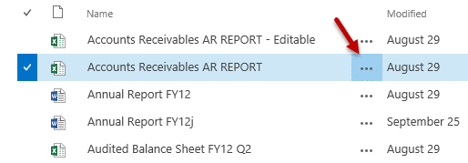
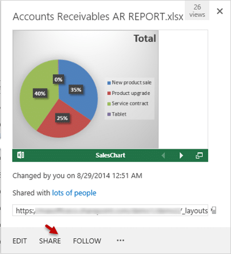
Once the file is in SharePoint you have to share it with the intended recipients of the report. Click on the option button (…) next to the file and choose Share – type names of people. Choose whether they can Edit or View and click Ok.
A preview of the Excel content is also shown in this dialog for your convenience. It also shows the views on the file!
How do the recipients get the report?
Once you send a sharing invitation, they will receive the link to your report by mail. The mail will be sent by SharePoint.
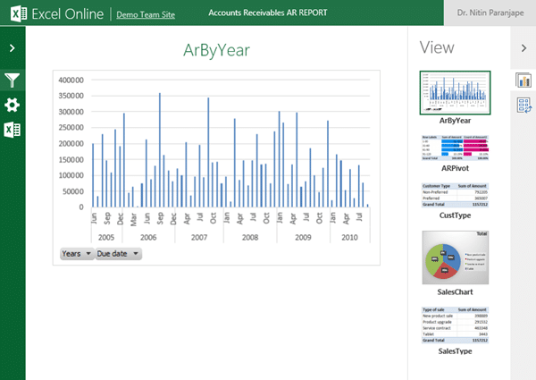
They just have to click the link. The items you chose to display will now be shown on the browser – in a nice scrolling menu.
On the right side – under the View area – small thumbnails of all selected items are shown. Click on the item to view it on the main area of the page.
If you have used Slicers – which is basically a filter, you can see the slicer on browser as well.
New way to publish reports
This is, of course, a new approach. It will need time for you and your organization to implement it. But why don’t you publish a few reports right away and try it out?
Over the next few articles we will cover more practical topics like difference between view and edit permissions, multiple slicers, versioning, notifications, combining multiple reports into one dashboard and auditing.
Related Articles
Part 1 covers the concept.
Part 2 (this article) shows the step by step process.
Part 3 covers Frequently Asked Questions.
***


