Fourth article in Error Handling (Background Error Checking or Green mark) series. Read these articles first to maintain continuity.
Auditors, Risk Managers, Everyone: Did you know? These green marks are WARNINGS!!
Green Marks Part 2: Formulas showing wrong results!
Green Marks Part 3: More error handling and Green Marks Part 4: Inconsistent Formulas

In this article, we cover the remaining three types of errors: Unprotected Formula, Formula refers to empty cells and Data Validation Error.

Unprotected formula

If you have not protected any sheet, this error will not appear. If you want to allow editing of specific cells, we need to protect the other cells. This is done in two steps.

1. Unlock the cells which you want to remain editable (Format Cells – Protection)
2. Protect the sheet (Review tab – Protect Sheet – type password)

Now only the cells which were unlocked are editable. This is usually required when you wan to send the file to others and ask them to fill in some data. This is a simple way to collection information from one or more persons.

Usually, we only want the other party to type data. We don’t want them to change the formulas. The cells which we need to unlock are VALUE type of cells – because we are asking for information.

Sometimes, by mistake, you may end up unlocking a cell which contains a formula. This is not what we want. The other person should not be able to edit formulas. Which cell is locked or unlocked is not visible. You have to see the checkbox in the Format Cells – Protection dialog to understand this.

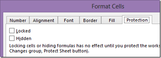
Therefore, you may miss the fact that a formula is editable even after Sheet Protection is applied. This is the time Excel shows our famous green mark. The error is Unprotected Formula.

The obvious action here is to Lock the cell. If for whatever reason, you want the formula to be editable, choose Ignore Error. In most cases you will want to lock cells. Therefore, you can select a range of cells and correct this error globally. To understand how to do this, refer to the article Auditors, Risk Managers, Everyone: Did you know? These green marks are WARNINGS!!

Formula Refers to Empty Cells

This option is NOT active by default. You must go to File – Options – Formulas – Error Checking Rules and activate this option. Here is an example of where this error can occur.

The data above and below is same. But look at the value of average function. It changed because the May value above was empty and the same value was Zero below.

Difference between Zero and Empty

I am sure all of us know this already. Empty and zero are two different things for Excel. Even from a business point of view, zero means we know that the value is zero. Empty value could mean that the data is not available yet for some reason. This ambiguity can lead to misinterpretation.

For example in the case above, if May was a month of vacation and there were genuinely no cases there, the average function should take into account the May value. On the other hand, if we were awaiting information about cases in May, the average should ignore the May value.

To highlight this ambiguity, Excel shows a warning – the green mark.

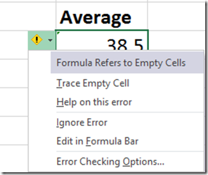
Unlike many other errors we have seen before, there is no corrective action possible here. It is your call. Trace Empty Cell is just a convenient function to help you identify where the empty cells are in the precedent ranges. In our example shown above, the formula and the data is near each other. Therefore, we can easily see the empty cell. However, if there is a complex formula where the data is in another sheet or far away from the data, you will need to know which part of the formula is referring to the empty cells. This is what the Trace Empty Cell feature does.

Consider the formula below. This is an average of four averages.

One of these ranges contains an empty cell. Green mark is shown. Trace empty cell option does not trace all the ranges. It only shows a red arrow which is pointing towards the range which contains empty cell(s ).

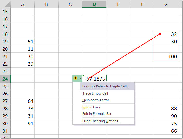
Once you identify the empty cell, the decision of whether to leave it empty or type zero or try to find the actual value, is up to you. This is dependent upon the context and your discretion.

If you are ok with the way empty cells are represented, choose the Ignore Error option.

The problem: All formulas are marked

This ambiguity about empty cell vs. explicit zero applies only to a few functions. Not all functions. Average() is one such function. However, for a large majority of commonly used functions, there is no difference between empty cell and zero cell.

Due to this, you may have to correct this error for lots of cells in a complex file. That is probably why Microsoft kept this option inactive by default. Ideally, this error should appear for only those formulas which treat zero and empty cells differently. But level of intelligence is not yet incorporated as of date.

This error CAN be ignored by selecting a range of cells or the entire sheet.

Understand this confusing setting

This sheet level setting in File – Options can create further ambiguity and visual confusion.

By default, this option is active. Which is good. IF there is a zero in a cell, it shows the value zero. Well that is what you would expect. Right?

However, if you clear this check box, the value of zero is also shown as blank. Now, visually a genuine blank and a cell which actually contains zero will look the same.To avoid this confusion, you should activate this option.

How to fill all empty cells with zeros

There may be situations where all the empty cells in a range (or a column) actually mean zero. How to fill all of them quickly with zeros? Here are the steps.

1. Select the range
2. Press F5 (Go To) and click the Special button
3. Choose Blanks and click Ok
4. Now all the blank cells within the range are selected
5. Type zero in the active cell
6. Press CTRL along with ENTER key (NOT shift ctrl enter. This is NOT an array formula)
7. Now all the empty cells are filled with zeros

The last error: Data Validation Error

This is the last error monitored by Background Error Checking in Excel. To understand how it works and what is the benefit, we must first understand what is data validation.

Here is a simple example. In this range I want to ensure that data must be between 50 to 100. I want to apply this validation BEFORE the data entry happens.
I am sure you already know how this is done using Data Validation.
If not, refer to this article.

Now, if I try to type data in this cell which is outside the bounds, an error message is shown.

Unfortunately, the error message does not SHOW what is the expected valid set of values. Therefore, if you created this file and sent it to others for data entry, you will have to spend additional time in showing the validation message. This message can be set using the Input Message tab in the Data Validation dialog. But this needs to be done manually for each validation. The benefit is that the message is shown as soon as you click inside the cell – providing clarity about the expected values.

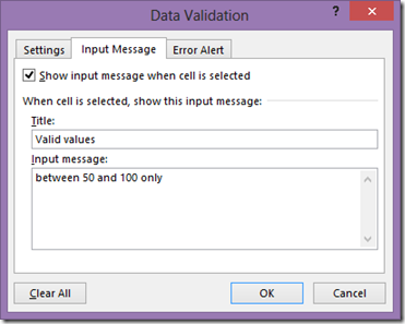
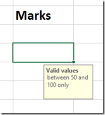
Make sure that the actual validation and the input message values match. Otherwise it will lead to confusion!

Validating data AFTER it is already entered

This is another common requirement. You have received data from someone and want to CHECK which are the values beyond the valid range (NOT between 50 and 100 in our example). To do this, you select the data and apply the validation. I have already applied the validation to the data shown below.

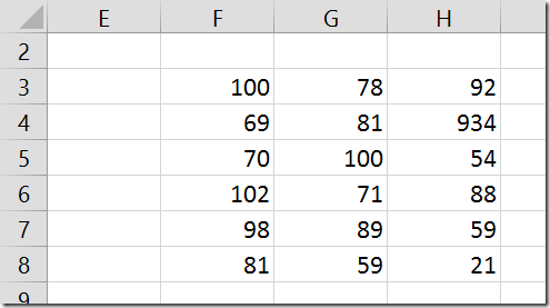
Obviously there are some values which are beyond our range of 50 to 100. However, there is no error message shown. Why is this so? Because, validation error message applies only if you edit the data. In this case the data has already been entered and the validation was applied retrospectively. Therefore it does NOT display any error message.

Does it not understand that some of the values are invalid? Of course it does. But it is not showing the problem values to you.

If you want to display the invalid values, choose Data – Data Validation drop down – Circle Invalid Data. This brilliant option has been there for a long time -but commonly missed.

Now the invalid values are shown. These circles do not Print. Only for display. If you change the data in an invalid (circled) cell, to a valid value, the circle will disappear. This way you can see the pending invalid numbers easily.

Although this is a good method, it requires manual intervention to activate the circle invalid data option. This is problem number 2.

Table and data validation

Without these red circles, it is not possible to view which cells are invalid. It is impossible to navigate the invalid values easily (if data is large).

Instead of showing the validation circles, now we have a much better option. Using Tables!

Here is the same data with the same validation – converted to a Table. Now see the difference. Cells which are invalid are already marked with our friend – green error mark!

Click inside the cell, open the exclamation mark dropdown and see the available options. Choose Display Type Information.

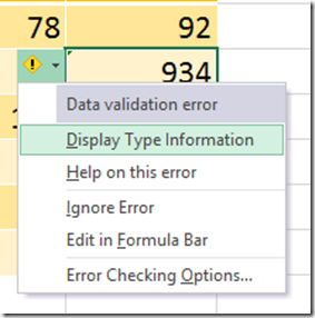
It automatically generated the appropriate description for what is a valid value based upon the validation rule. Nice and useful.

Summary

That brings to the end of a 5 part series on Background Error Checking feature of Excel. As you can see, it is a very important and critical feature. Now you have all the knowledge required to notice, interpret and handle all the errors indicated by Excel.

Please share this series of articles with everyone in your organization to ensure accuracy and reduce risk of misinterpretation / wrong decisions.

CNN article: May be we can now understand what happened

I just came across this article on CNN: Damn Excel! How the ‘most important software application of all time’ is ruining the world

It highlights many famous people / situations which occurred because of errors in Excel. Now that you have gone through this series of 5 articles, you can imagine where the real problem lies.

The ignorance about effective usage of Excel (for that matter – any technology) is so rampant that it is not even being noticed as a problem. Sad and dangerous. But true!

***