All of us use the Filter area in Pivot Tables. Do you know there is a more powerful way that has been available for 5 years? Learn it and use it.
Estimated reading time 10 min
This article applies to Excel 2010 and above.
Contents
Download sample file and follow along
Sample Data sheet contains raw data. Each row is a transaction. I have removed unwanted columns.
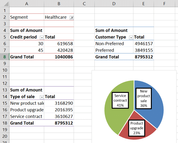
Second sheet is named Dashboard. It contains a manually created dashboard. There are three pivot tables and one pivot chart. One pivot was created from the raw data and others were copy pasted. One pivot table has a filter on the Segment field.
The problem with Pivot Filters
- Each pivot requires its own filters
- Filters need to be synchronized manually
- Multiple selections are not visible
- Filters don’t filter each other
Each Pivot table requires its own filter
This is obvious. There are four areas available for each Pivot Table. Rows, Columns, Data (Values) and Filter.
Our dashboard contains multiple pivot table. Only the first Pivot Table has a filter on Segment column (Healthcare).
Now you can appreciate the problem. The first pivot is filtered and all other pivots are showing the whole data (across all segments). This is misleading and confusing.
Ideally we want the same filter to be applied to all Pivots and Charts.
How do we do that? Unfortunately, by manually going to each pivot table and adding the same Segment column again and again (three times in our example).
This is just the beginning of our misery.
Filter Synchronization?
Just adding segment to each pivot table is not enough. Each filter must use the SAME filter condition. Which means the selection of the segment (Healthcare) must also be done thrice in this case.
If the segment is changed in one pivot, it has to be repeated for all pivot tables .. again and again.
Multiple selection of filters
Open the filter dropdown and choose the Select Multiple Items checkbox. Select multiple segments – Healthcare, Telecom and Retail. Click Ok.
Once the selection dialog closes, there is not enough place to show all the filter conditions. Therefore, Excel shows an ambiguous thing called Multiple Items. The only way to know the ACTUAL filter condition is to open the dropdown and look.
Filters are not filtered by each other
Consider we have two filters. Segment and Month. Both filter dropdowns will show all items. Sometimes there is no data for a specific segment in a specific month. Even then both items will be shown. That means the first filter is not filtering the second filter.
The only way to know that there is no data is to select both filters and then notice that the pivot table is empty!
Solution to all these problems is called a Slicer
This was introduced since 2010 version of Excel.
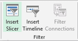
Click inside the pivot and choose Analysis tab – Insert Slicer
For Excel 2010, use the Options tab.
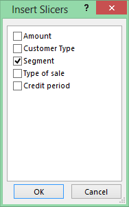
Now a list of all available fields is shown. Choose Segment.
A floating window appears showing all segments. That is the Slicer. It will overlap the Pivot Tables initially. Add few columns between the two pivot tables and readjust the size of the slicer window so that the scroll bar is not required.
Notice that the slicer is also showing the segments we chose earlier – Exports, Healthcare and Telecom. Blue items are the current filters.
Now we don’t need the Segment field in the filter area of the first pivot table. Slicer will do all the filtering for us. Click inside the first pivot and drag out the segment column from the filter area.
Using Slicers
Click on the remove filter icon in the title bar of the slicer. This will clear all filters. All segments are now selected indicating that there is no filter.
To select a segment click on it. Ctrl click also works. Drag selects multiple items. Change the filter and see which pivot tables are affected.
Unfortunately, only the first pivot table is getting filtered. Why? Because we clicked inside the first pivot table and added the filter. Therefore, it is linked only to that pivot table.
Linking the slicer to multiple pivot tables
Don’t worry. Slicer is capable of handling multiple Pivot Tables. Click on the Title bar of the slicer (on the word Segment). On top – in the ribbon – a new tab called Slicer Tools will appear.
Look for an option called PivotTable connections (Excel 2010) or Report Connections (Excel 2013). Now a list of all pivot tables which share the same data are shown. Select all of them.
The pivot table names are not very intuitive. Ideally each pivot table should be given a relevant name. Analyze tab (Options tab in 2010) – on the leftmost side of the ribbon Pivot Table Name can be changed.
Now try the slicer again. All pivot tables (and pivot charts) are now filtered in a single action. There is no need to filter three times!
Frequently asked Questions
Yes. More than one slicers can be added.
Yes. Slicers work on a browser page when saved to SharePoint.
Yes. Slicers work on iPad, Android tablets and their respective browsers also.
Homework!
Try slicers on your existing pivot tables.
Consider how existing reports can be enhanced and made more flexible using Slicers
If you have never created multiple pivot based dashboards, now is the time to do it.
What Next
In the next article we will see how Slicers filter each other.
***


