This is the continuation of data cleanup series. In this article we discuss a newly introduced feature “Flash Fill” which is almost miraculous and difficult to believe. When I demonstrate this feature during my seminars, most people suspect that I am playing some kind of trick!
It opens up a new way of handling data cleaning tasks which would have either been very time consuming or impossible using existing methods.
This feature works only with Excel 2013 and later.
Contents
Data cleanup example
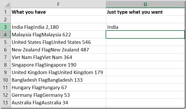
The best way to learn this feature is to see it in action. Consider this data. It contains three columns in a single column. Ideally we would just want to split it into TWO columns, one containing the country and the other containing the number.
Where did this data come from? Obviously, it was copy pasted from some web page where there was a flag image shown next to each country. While pasting in Excel, someone chose past as plain text – and this is what we got.
Usually we will try Text to Columns – but it will not work here. The spaces are uneven as some country names are single words and some are two words.
Here is where Flash Fill Shines. Go to the next column and type what you want. No need to put a formula. No need to select the data range. Just type.
Nothing sensational happened. Don’t worry. Go ahead and type Malaysia – and see what happens.
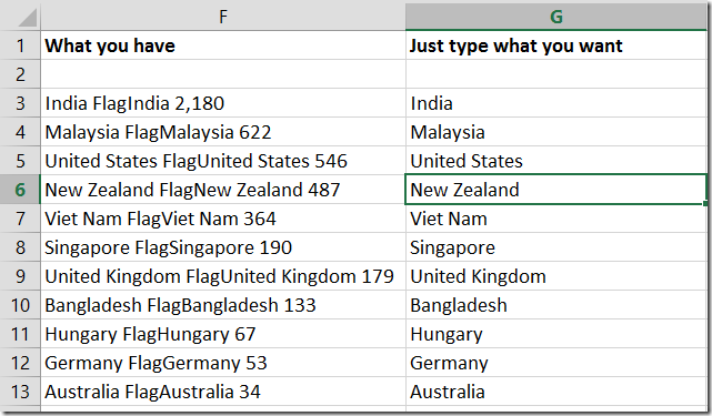
The moment the M for Malaysia was written, Excel automatically understood what you are trying to do. It figured out how to do it and it is suggesting that if you press Enter now, all the other names will be automatically filled.
Press Enter and see what happens. Obviously it is not doing its job very well. It only picked up the first word from two word country names. Problem…
Don’t worry, go ahead and change United to United States and see what happens.
Now it is perfect. It required two examples because there were two patterns in the data. One word countries and two word countries. Is that not smart?
Validate the automatic fill
Notice that small icon which appears. When you open it, you will see more useful stuff. When you changed the entry for United States, the logic was applied to all the rows but only three rows changed. From this menu you can choose and see which rows changed. This helps you confirm that the desired result has been achieved.
In this case the data is small and you can see it at a glance. However, while handling big amounts of data, it is important to highlight the affected cells and check if the output is correct.
Splitting the next column
But wait, we also need the number. So what next?
Go to the next column and type the first number 2180, then 622 and then 546. Now it detects the pattern. Press Enter to fill all rows.
Do it manually using Flash Fill button
Notice that in each case, you had to provide 2 examples before the pattern was detected. If you want, you can ask Excel to perform this automatic fill after providing just one example.
For example, in the above example, just type 2180 and then choose Data – Flash Fill button. This forces the Flash Fill to occur with just one example.
The science behind this feature
This great feature is based upon a very complex pattern matching algorithm (regular expressions). The original work was done at Microsoft Research by Sumit Gulwani. The paper is titled Automating String Processing in Spreadsheets Using Input-Output Examples. Those of you who are academically interested can Download and read the paper.
What next
Try this feature in your day to day work. In the next article, we will cover more interesting variations of Flash Fill functionality.


