Excel IF function – Dos and Don’ts

So far, I have not written an article about the humble IF function. But in the last few months I came across many customers who asked me to explain how the IF function works. Surprised? The reason is that many people use the Excel IF function, but they do not understand its nuances.

Usually someone has created a file and is handed over from person to person. Worse still, those who know how to use the IF function misuse it! So here it is a simple, short and practical description of how to use the IF function.

Excel IF function

The Need

Working with data requires decisions to be taken. Usually decision making has a basis. In terms of Excel, there could be one or more conditions which can lead to a decision. Depending upon whether the condition is met with or not, we want to take different decision. This is where the IF function in Excel is very useful.

How to check if B2 is greater than the Benchmark?

Let us start with a simple example. We are conducting a test on a product.
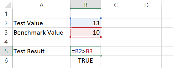
We want to know if B2 is greater than the benchmark (B3).

This requires a very simple formula as shown below:

= is just to start the formula entry.
Thereafter we are checking if B2 is greater than B3. No Excel function is required.

This formula is like asking Excel a question, “Is B2 greater than B3”? Now, Excel must reply as Yes or No.

Excel is not a human being so it answers in a technical way as TRUE which basically means Yes. If B2 is lesser than or equal to B3, Excel’s answer would be “No” which is shown as FALSE.

If we just wanted to know this information, we have already finished our job.

Take an action, based upon the comparison

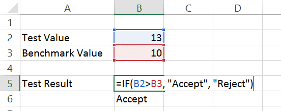
If B2 is higher than the benchmark, we will accept the product, otherwise reject it because it failed the Quality Check. This is where the IF function is used.

Here is another variation.

How does the IF function work?

IF function is just emulating our decision basis. Because it is a function, you must communicate with it by providing relevant data to it.

1. The first parameter is the basis of our decision or the condition.
2. Second parameter is to specify what to do if the condition is TRUE and
3. The third parameter is to say what to do if the condition is FALSE.

While typing the function, this syntax is shown for your reference.

Notice that the cursor is positioned inside the comparison. That is the logical_test parameter. Other two parameters are called value_if_true and value_if_false.

That’s it. Practice it a few times and you will get the hang of it.

What kind of logical test works?

Well, practically any formula will work as a logical test. It should return TRUE or FALSE.

In fact, even non-logical data can also be put as the logical condition.

This formula will always return True Value as the result.
Any positive number is considered as logical TRUE. Zero and below is considered as logical FALSE. That is how the Excel IF function works.

More complex decisions using Excel IF function

Let us go back to our Test results example.
Suppose if the test value is above the benchmark, we accept the product.
If it same as or 2 below the benchmark (between 8 and 10) then we must retest.
If it is below benchmark – 2 (less than 8), then we should reject it.

How does this work?

Look at the Formula syntax below the formula itself.

First IF condition checks if the test value is higher than the benchmark. If TRUE, we Accept.

Now we have one more condition to test – is it higher than 8 or lower than 8. That is being done in the second IF statement. The entire second IF statement is a part of value_if_false part of the first IF statement. Thus, if the first if fails, it tries the second if and returns the desired decision.

Caution: Too many IFs are usually bad

We saw that with three conditions to check against, we needed two IF statements – one inside the other. What if you had multiple such conditions to check – for example 0 to 2, 2 to 4, 4 to 6 and so on? You will find it very confusing and cumbersome to put IF statements within each other.

We still get the formulas right – somehow. But usually, if there are many such conditions required, VLOOKUP function is a better choice.

Another misuse (and overuse) of related functions like COUNTIF(), SUMIF(), etc. is also a common occurrence. Often, the simpler solution is to use Pivot Tables.