 |
If you use text month in a Power Pivot Table, it is sorted in alphabetical order.
Here is the solution to the problem. Quick Solution time 2 min
|
Contents
This is my 400th article!
The Problem
Suppose this is the raw data in Power Pivot Data Model.
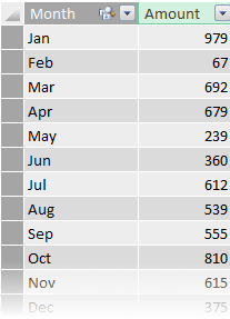
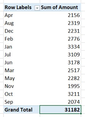
The Power Pivot table contains the same two columns. It will calculate total amount for all months. The problem is that the months are ordered in alphabetical order – not Month order (Jan, Feb, Mar, …).
If you make a regular pivot table with exactly the same data, it will understand that those are months and order it automatically. This happens because Excel already has a built-in Custom List which defines the order of months.
Quick Solution 1
Manually use the custom list sort order. Right click in the month column and choose Sort – More Sort Options. Choose the Custom list and that’s it.
Quick Solution 2
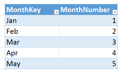
Add a master table (called Months here) containing 12 rows – one for each month. First column contains MonthKey – which is just the text month. Add another column called MonthNumber which simply contains serial numbers as expected.
Create a relation between original table Month column and MonthKey column. Now select the Months table and choose Sort by Column as MonthNumber. Use the MonthKey column in the actual Power Pivot. It will be sorted automatically in the right order.
Download File and follow along
What is in the file?
Two sheets. Sheet1 contains raw data in two tables Data and Months. Both tables have already been imported to the Data Model.
The second sheet contains the Pivot table created from Power Pivot.
Detailed Solution 1
This is a quick and easy way. Although I would recommend that you should use the second solution – because it is more elegant and will help you with many more time related things.
Go to the Power Pivot sheet. Click inside the pivot table. The Field list will appear. Notice that the month column is taken from the DATA table. The sorting order is alphabetical.
Changing the sort order
This is quite easy. This happens automatically in regular Pivot Table. In case of Power Pivot we have to the sort order manually.
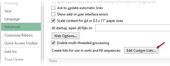
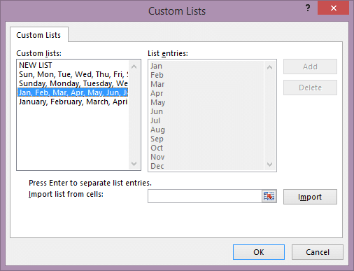
First of all, notice that there is a pre-created custom list in Excel for all months and days. To see it choose File – Options – Advanced – scroll all the way to the bottom and click the Edit Custom Lists button.
Existing custom lists are shown. Remember that new custom lists can be created and used by importing existing data or simply by typing a new list in the dialog directly.
The four built-in custom lists cannot be edited.
Click Cancel. This was just to make you aware of this feature. Here is a detailed article on using custom lists: Custom sorting in Pivot Table using Custom Lists
Custom Sorting Order in Power Pivot
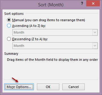
Come back to the Power Pivot table. Right click in the Month column and choose Sort – More Sort Options. A complex looking dialog appears. Don’t worry. By default Pivot Table sorts things in their natural order depending upon the type of data. However, Sorting order can be manually changed by dragging the actual item in the row or column area. But for now we don’t need this option (this requires another article actually!).
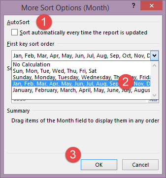
Choose More Options. Now another dialog opens – which is equally confusing!
Unselect the Sort automatically… option. Now the First key sort order option will be active. Choose the Jan, Feb, Mar, … custom list. Click Ok and close all dialogs.
That’s it. Now the sorting order is appropriate. Problem solved.
Same concept can be used for days of week as well.
Next article
In the next article we will see another solution which uses Power Pivot feature of determining sort order by default whenever any field is added to pivot table.
***

