Yes. This is a simple rule of efficiency. Of course, this rule is in the context of Office tools. But you never know, try applying it to real life – may be it is equally useful there. Using the example of GetPivotData – we will learn this concept.

The concept

There are many features which irritate us. Obviously, nobody wants to create features which irritates customers. Microsoft takes extreme care to make the User Interface as easy to use as possible.

Most people will laugh at me for saying this – because the usual perception is that Office is too complicated and feature laden. But never mind that. Some other time.

If users do not like a particular feature, the creator should remove it and reintroduce it in some more palatable way. Microsoft has refined, removed and added thousands of features based upon user feedback.

But in spite of that, some features irritating features are still lingering. One example is GetPivotData.

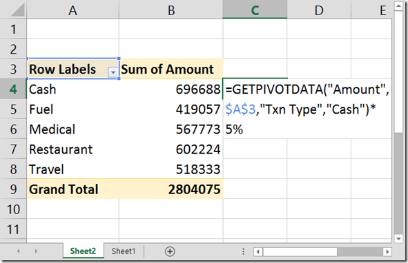
Whenever you try to put a formula which refers to Pivot Table data area, this irritating function is automatically added by Excel.

Nobody knows why it comes and nobody cares as to what the benefit is.

Guaranteed irritation – NO benefit.

Why does Microsoft want to irritate billions of users?

This is a very important question. Of course they know that people don’t like GetPivotData. But they have kept it for more than a decade. Why? Why? Why?

The only answer possible is : The feature is EXTREMELY USEFUL.

So Microsoft is hoping that even if you are irritated with it, some day you will explore what it does and then you will benefit from it.

What is the purpose of GetPivotData?

Often, we need to put formulas based upon data shown in a Pivot Table. The function appears automatically. Let us say we want the revenue for Malaysia for Master card.

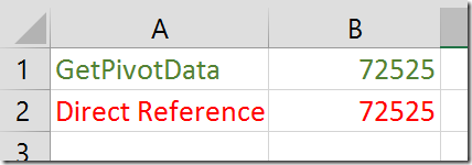
For now, let us just accept what the formula says. Press Enter. It does show the value 58592.

Most of us are not going to press Enter but press Escape! And add the formula manually, as follows…

This also shows the same amount

So far so good. Remember – the top one is GetPivotData based (Green) , and the lower one is a direct reference (Red).

So what is the difference?

Right now there is no difference. But now watch.

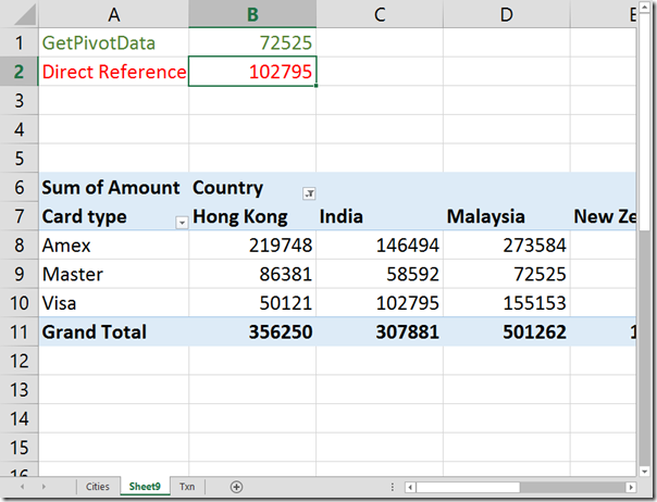
I am swapping the rows and columns of the pivot table. see what happens.

GetPivotData is still showing the right answer. Whereas our hard-coded formulas is blindly showing whatever is there in C10.

That is the difference.

GetPivotData always returns accurate results!

Now let us try another thing – which will make things fail.

Let us remove the card type altogether from the pivot table. But even now, GetPivotData wins over the direct reference…

GetPivotData shows a proper error – indicating that the information in the Pivot is not sufficient to get the results. The direct reference fails miserably – again!

The syntax

GETPIVOTDATA( data_field,  pivot_table,  [field1, item1, field2, item2], …)

It looks complex, but it is actually a very simple syntax.

First is the data column to use in the aggregation, in this case the Amount column.

Second parameter is the identifier for the pivot table. Usually the top left cell of the Pivot Table is used here. However, technically it could be any cell within the pivot table.

Now there are pairs of Field and Item, Field and Item and so on…

These pairs describes what we want – like Country = India and Card = Master…

If you do not specify any Field – Item pair, then the output gives you the grand total.

Writing this syntax by hand would be very difficult. That is why Excel auto-generates it and gives it to you.

Bottom-line: Point references to data area in Pivot Tables should always use GetPivotData

Try it out yourselves and see how useful it is.

Another problem, and solution

Often we try to use a formula along with GetPivotData function and then drag it down to copy the formula. Unfortunately, it gives the SAME result. Don’t get frustrated.

As you have seen, GetPivotData returns a single value based upon the Field-Item pairs. Therefore, even if you drag it down, the value is same – that is why the formula results are the same.

If you really want it, you can change the item value from the hardcoded value to a variable value. This way you can drag a formula and get the desired results.

However, I would not recommend this unless there is no way of doing it within the pivot table.

Using hard coded formulas referring to Pivot Table data are very risky and error prone.
Always use GetPivotData.

Problem

Now that you understand the importance and benefit of using GetPivotData, you will want to use it for more than one cells. Unfortunately, GetPivotData syntax gets generated one cell at a time. You will have to go to each cell one by one – which is a very tedious process.

To solve this problem, we (me along with my friend Raj Chaudhuri) created a nice little macro called pastepivot. Read this article to download the macro file. Usage instructions are also included in the article. Paste Special Pivot – New way to use Pivot table data.

Enjoy